Trees and networks
It’s been over a month since our last post and for that we must apologize. We endeavor to be more prolific, but sometimes work and life get in the way. On the work front, let’s just say we won’t have to spend as much time selling encyclopedias door-to-door, which should free up more time to dedicate to writing value-added blog posts. On the life front, we had the chance to hike several canyons in southern Utah, USA. Our favorite was the slot canyons of Escalante; Antelope Canyon in Page, AZ was pretty awesome too.
Now that we’re back in the saddle let’s get back to important stuff like neural networks! In our previous posts, we compared linear, logistic, and multinomial logistic regressions to neural networks. In this post, we’ll run similar comparisons on decision trees.
One of the great things about decision trees is they make no assumptions about the underlying distribution of the data. Moreover, they’re relatively easy to explain to the lay person; that is, until you start talking about Gini impurity or entropy. Even then, with a little hand-waving, it’s somewhat straightforward to give one a general idea.
How do decision trees work? They search for a feature and a threshold of that feature such that splitting the data along this threshold produces the greatest “purity” in each subset. Ok, but how does it do that? It minimizes the impurity of each subset. Uh, ok.
Think about it this way. Let’s take the classic dog example from our last post. We’ve got Pekingese, Poodles, and Shih-tzus with a bunch of data around tail length, nose length, height, weight, etc. If we had 50 varieties of each dog, and found some feature, f, whose value, v, above which only Pekingese were found and below which were the remaining Poodles and Shih-tzus, that would seem like a pretty good threshold. This would allow us to put all the Pekingese in one bucket (or node in tree speak1) and then look for other features and thresholds to split the Poodles and Shih-tzus.
What’s the impurity for the node that has all the Pekingese? Zero because all the labels in that node are the same. A zero impurity yields a high purity in the double negative logic of statistics. Mathematically, it looks like the following
\(G_{i} = 1 - \sum^{n}_{k=1}p_{i,k}^{2}\)
Where, \(G_{i}\) is the impurity of node \(i\) and \(p_{i,k}\) is the ratio of instances of class \(k\) in the \(i^{th}\) node. As the sum of the ratios increases, impurity declines at an increasing rate. In other words, as more of the same instances are put into the same bucket, the purity of the node increases at a faster rate.
The cost function the algorithm minimizes is the weighted average Gini impurity of the split. This is given by
\(J(k, t_{k}) = \frac{m_{l}}{m}G_{l} + \frac{m_{r}}{m}G_{r}\)
Where \(k\) is the feature and \(t_{k}\) is the threshold of \(k\), \(m\) is the number of instances across the subset, \(m_{l}\) and \(m_{r}\) are the number of instances in the left or right subset, and \(G_{l}\) and \(G_{r}\) are the Gini impurity of each subset.
The algorithm searches for the best split among all features at the outset and then repeats for all remaining features unless specified. It doesn’t look for the best combination of splits or the highest purity after a certain number of nodes. This means it it unlikely to find the an optimal combination of splits, but will likely find reasonably good ones.
As mentioned above, entropy may also be used. The concept comes from physics, but has also been applied to information theory. Less order—in molecules or information—means more entropy. The Entropy equation is:
\(H_{i} = -\sum_{k=1}^{n} p_{i,k}log_{2}(p_{i,k})\)
Here, \(p_{i,k}\) is the same \(p_{i,k}\) from above. The negative sign reverses the impact of taking a log of a fraction. As \(p_{i,k}\) gets close to 1, the log gets close to zero, meaning entropy declines.
Apparently, it usually doesn’t make a huge difference in results whether the decision tree uses Gini impurity or entropy, at least according to different researchers.2
The nice thing about decision trees is that they approximate rational decision-making when faced with several choices. First, look for the feature that is likely to have the biggest difference in outcomes and then go through the remainder until you’ve exhausted a good range of likely outcomes. The difference, of course, is that the outcomes are already known with decision trees.
How does this relate to investing? Google scholar finds over 90k articles on decision trees and stock prediction. Using decision trees to parse lots of disparate data to figure which features seem to have the greatest impact without having to make lots of assumptions about the underlying distributions seems like a relatively intuitive way to construct a good first pass analysis. Let’s throw some data at this puppy and see what we find.
In our previous posts, we were using the monthly returns and the ten-month moving average of those returns on the S&P 500. We’ll complicate things by using more stocks, which should motivate some of the additional analyses we’ll conduct later as we compare more complex structures. We pull the monthly returns from 2010-2020 on the thirty stocks in the Dow Industrial Average as of the end of April 2021.
For each stock we generate a rolling average of monthly returns for the last two to twelve months—11 series in all. We then standardize these returns for each date across all the stocks on that date. These will be our features. For our labels, we calculate the return in the next month for each stock and convert that into a binary outcome: 1 for positive returns, 0 for negative. (We opted for decision tree classification to make the explanation more straightforward. Regression is an option too.)
Next we form the train, validation, and test sets by splitting according to the following proportions: 60%, 20%, and 20%. We run our first decision tree with a relatively simple structure—only two nodes, aka a max depth of two.3
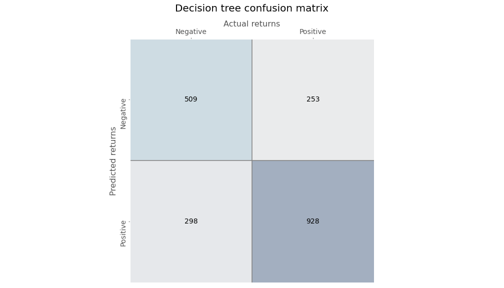
Running the algorithm, we parse the predictions into our trusted confusion matrix below to see the results.
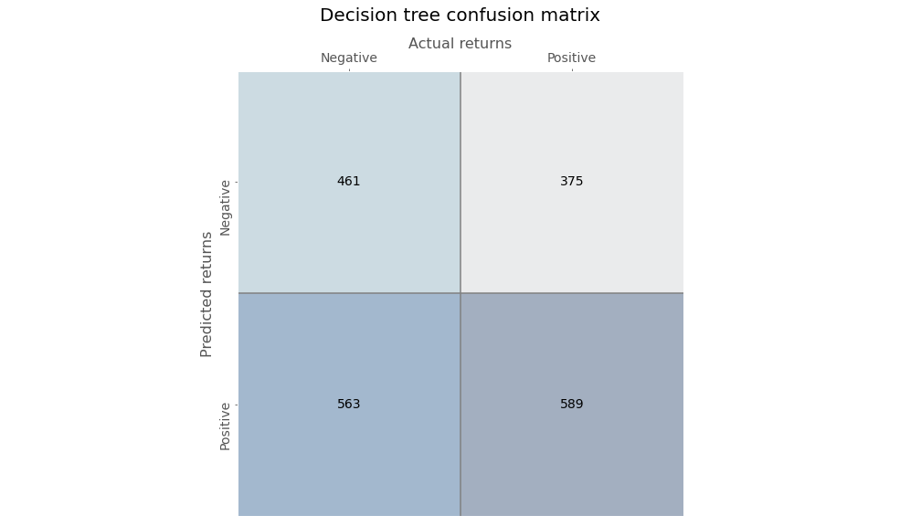
Not very impressive. The accuracy is only slightly better than a coin flip. Precision is also 50/50. But recall isn’t bad. The true positive rate is definitely better than the true negative.
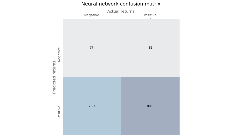
Now we’ll train a very simple neural network using only one output layer with a sigmoid activation function to assign probabilities. Here’s the confusion matrix for the neural network.
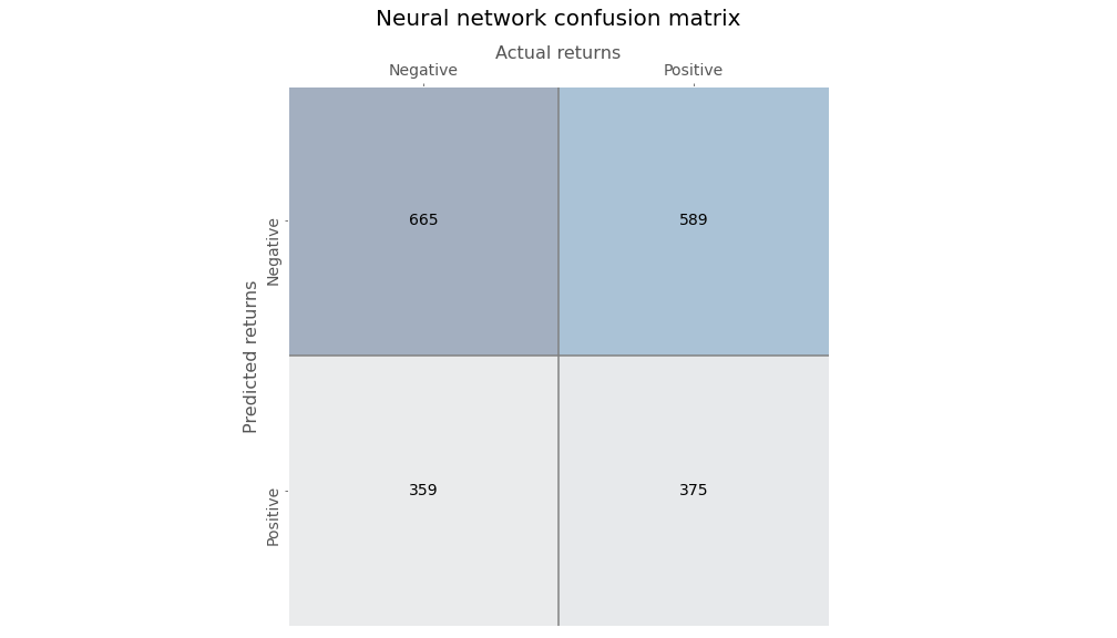
The neural network’s predictions are more biased than the decision tree, skewing toward negative returns. Precision is not much better than random and recall is poor too.
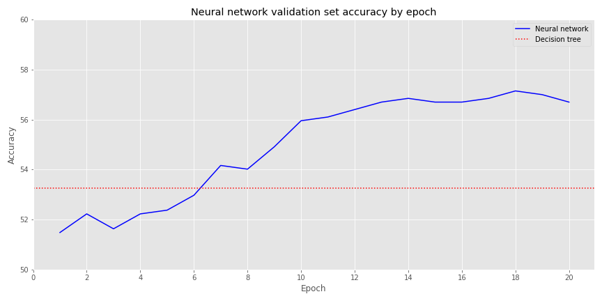
Out of curiosity, let’s see how the accuracies compare. In the graph below we chart the accuracy of the decision tree vs. the neural network (NN) over its various epochs for the validation set rather than training to see how things look out-of-sample
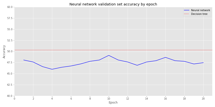
The NN’s accuracy isn’t dramatically lower than the decision tree’s. But investing in these results would probably have an expectation little better that roulette! While this is a nice warm-up, it’s now time to get serious.
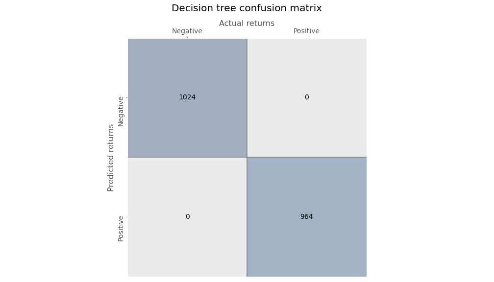
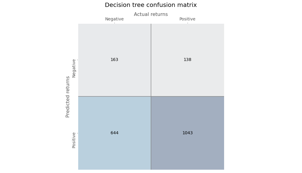
We create a decision tree without a limit on the number of branches it can grow, meaning that it will continue growing until all the leaves are pure or contain less than the minimum sample, which is two in this case. When we do that we get a perfect model: every down and up month is accurately bucketed—a clear sign of overfitting.
In contrast, we create a slightly denser NN with two hidden layers of 30 neurons each and the same fully connected output layer. On the training set, the NN’s accuracy significantly underperforms the decision tree, as show in the graph below. No surprise there.
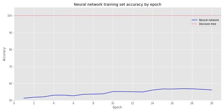
But when we look at the validation set, performance flips. The decision tree’s accuracy is actually less than 50% and the neural network’s is about the same as the training set.
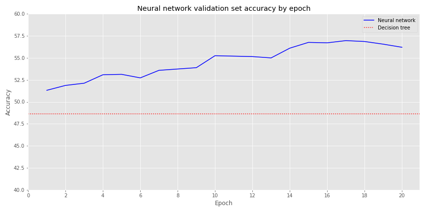
Overfitting is a well-known drawback to decision trees as we saw play out above. Generally, one would regularize the hyperparameters using some form of cross-validation or prune unnecessary nodes to overcome the issue. But we’ll save that discussion for another time.
Let’s create a series of momentum risk factors based on the different rolling periods similar to Jegadeesh and Titman. For instance, we’ll have a risk factor for the two-month, three-month, all the way to the twelve-month rolling average of returns. We’ll build this risk factor by ranking the cross-sectional rolling average of returns for the Dow 30 stocks, construct portfolios from the top and bottom deciles, and subtract the bottom from the top.
The two-month momentum risk factor looks like the following:
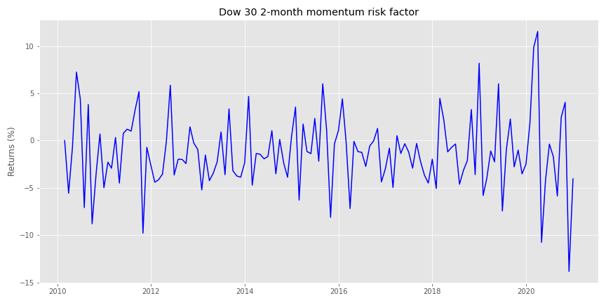
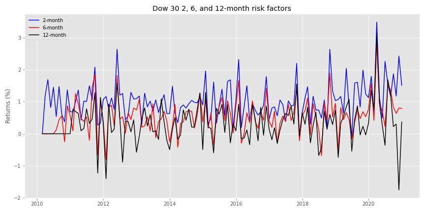
Here’s a spaghetti chart of the two-month, six-month, and twelve-month risk factors.
Note, in our first pass, we won’t normalize the factor returns, but we’ll continue to look at the forward returns for all of the stocks. We’ll construct a decision tree classifier once again, but we’ll use a max depth of four nodes to prevent egregious overfitting. Here’s the confusion matrix.
Precision and recall are both in the high 70% range, which is pretty good. The false positive rate is pretty good too: in the mid-30% range.
We’ll use a similar neural network architecture as before: two hidden layers of 30 neurons each, and a final output layer with a sigmoid activation function. When parse the model’s prediction on the training set we get the following confusion matrix.
Recall is quite high (above 90%), but precision is lower (at 60%). The high true positive rate is mostly offset by a high false positive rate too.
We won’t show the confusion matrices for the validation sets, but will show a performance metric summary and the accuracy comparison graph.
| Model | Recall/True positve rate | False positve rate | Precision |
|---|---|---|---|
| Decision Tree | 57.4% | 52.7% | 61.4% |
| Neural network | 91.2% | 93.8% | 58.7% |
Interesting, by the sixth epoch the slightly dense neural network is already outperforming the decision tree, though not dramatically.
There’s a couple different ways to go from here. We won’t pursue all of them since we don’t want to turn this post into an exhaustive exposition.
We run a grid search cross-validation to find the best set of decision tree hyperparameters—the details aren’t overly important; you can check the code below if interested. Using these best parameters, we re-run the model and reveal the following confusion matrix.
Recall is fairly high (high 80% range), precision is ok (around 60%). Unfortunately, the false positive rate is rather high too (near 80%). Still there isn’t a huge diminution in accuracy between the training and validation sets (not shown), as both are close to 60%.
We’ll now build a relatively dense NN with some regularization to prevent overfitting. Regularization can get pretty complicated, pretty quickly and a bit ad hoc, so we won’t go into detail here; that deserves a post on to itself. Briefly, we drop some of the neurons between layers. By doing this we force some neurons to work harder and pay attention to more of the input neurons to find the best weights to produce the desired output.4 We could, of course, employ a grid search on the neural network too, but that’s a bit trickier and beyond the scope of this post.
We build a neural network with three hidden layers of 500, 250, and 100 neurons, dropping 20% of the neurons after each layer. We run 50 epochs, generating the following accuracy graph on the training set.
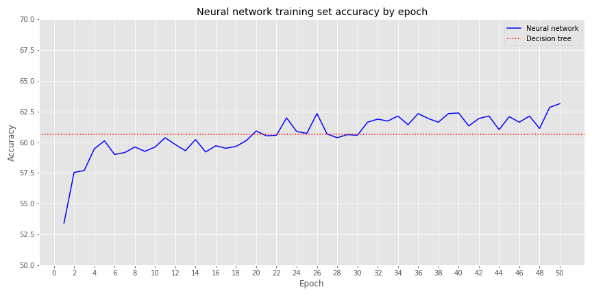
After about epoch 20, the neural network starts to outperform the decision tree, though generally not more than by a few percentage points. Let’s compare results on the validation set.
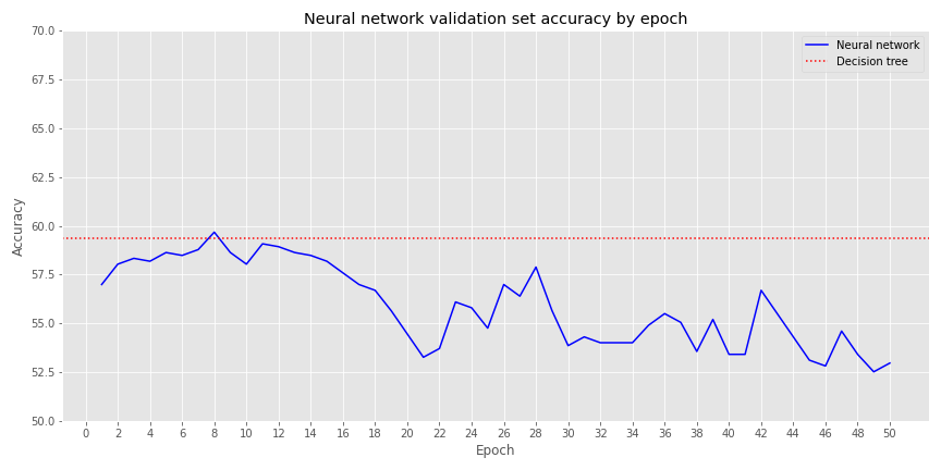
By epoch 8 the neural network converges with the decision tree, but it suffers poor performance thereafter. Let’s compare some of the performance metrics between the decision tree and the neutral network on the validation set. Recall, we’re using the best performing model from our grid search cross-validation on the decision tree. For the neural network we’ll stop the training right where it converges with the best decision tree model on the validation set, around epoch 8.
| Model | Recall/True positve rate | False positve rate | Precision |
|---|---|---|---|
| Decision Tree | 87.2% | 81.3% | 61.1% |
| Neural network | 95.5% | 92.7% | 60.1% |
We see the NN has a better true positive rate (TPR) than the decision tree, but its false positive rate is higher too. The better TPR comes at the expense of precision, which is actually lower than the decision tree.
Let’s sum up. Like linear and logistic regressions, neural networks can approximate the results of decision trees. But performance is not quite the same on several metrics. In many cases, the neural network outperforms the decision tree on the validation set, suggesting it generalizes a bit better. However, when we regularize the decision tree using cross-validation, that performance advantage disappears. We didn’t perform cross-validation on the neural network, so the comparison might not be fair. Still, as we’ve noted before, prediction is only part of the analysis. We’d want to test both approaches on model portfolios analyzing the risk-adjusted returns.
Whatever the case, explainability remains an open question. Linear and logistic regressions are relatively easy to explain visually. Decision trees are pretty good too, although we didn’t provide a graph in this post due to some technical issues. Of course, in this example, it’s not immediately intuitive why the best performing decision tree splits on one particular moving average or another. Nonetheless, at least you know where the splits occur, unlike with neural networks, which are pretty opaque as to why the weights on the neurons turn out the way they do.
In upcoming posts, we may run these analyses again on normalized risk factors, on decision tree regressions, and/or move on to random forests. We also plan to look at applying the decision tree vs. neural network comparison to financial statements. If you have preference as to which topic we tackle first, send us an email at the address below. Until next time, here’s the code you’ve all been waiting for.
 Built using R 4.0.3, and Python 3.8.3

# [R]
# Load libraries
suppressPackageStartupMessages({
  library(tidyverse)
  library(tidyquant)
  library(reticulate)
})

# [Python]
# Load libraries
import warnings
warnings.filterwarnings('ignore')
import numpy as np
import pandas as pd
import statsmodels.api as sm
import matplotlib
import matplotlib.pyplot as plt
import os
os.environ['QT_QPA_PLATFORM_PLUGIN_PATH'] = 'C:/Users/user_name/Anaconda3/Library/plugins/platforms'

plt.style.use('ggplot')
plt.rcParams['figure.figsize'] = (12,6)

# Directory to save images

DIR = "your/image/directory"

def save_fig_blog(fig_id, tight_layout=True, fig_extension="png", resolution=300):
    path = os.path.join(DIR, fig_id + "." + fig_extension)
    print("Saving figure", fig_id)
    if tight_layout:
        plt.tight_layout()
    plt.savefig(path, format=fig_extension, dip=resolution)

## Pull data
dow_30_ls = ['MMM', 'AXP', 'AAPL', 'BA', 'CAT', 'CVX', 'CSCO', 'KO',
           'DIS', 'DOW', 'XOM', 'GS', 'HD', 'IBM', 'INTC', 'JNJ',
           'JPM', 'MCD', 'MRK', 'MSFT', 'NKE', 'PFE', 'PG', 'TRV',
           'UNH', 'VZ', 'V', 'WMT', 'WBA', 'UTX']

dow_30 = dr.DataReader(dow_30_ls, "yahoo", "2009-12-01", "2020-12-31")['Adj Close']

dow_30.to_pickle('dow_30.pkl') # save for later!

df = dow_30.resample('M').last().pct_change()[1:]

### Create rolling mean return dictionary
# Create dictionary of rolling mean returns from 2 to 12 months

df_dict={}

for i in range(2,13):
    df_dict['df_{}m'.format(i)] = df.rolling(i).mean()

#### Create dictionary of cross-sectional ranking for each rolling mean period

df_ranks = {}

for key in df_dict.keys():
    df_ranks[key] = df_dict[key].rank(axis=1)

#### Creating risk factor for each ranking

df_mo = {}

for key in df_ranks.keys():
    top = np.where(df_ranks[key] >= 27,1,0)
    bot = np.where(df_ranks[key] <= 3,1,0)
    df_mo[key] = (df * top).mean(axis=1) - (df * bot).mean(axis=1)


# Graph risk factors: Used later in the post
import re
plt.figure()

keys = ['df_2m', 'df_6m', 'df_12m']
styles = ['b-', 'r-', 'k-']
months = [re.sub(r'[A-Za-z\_]+', '', x) for x in keys]
for i in range(3):
    plt.plot(df_mo[keys[i]]*100, styles[i])

plt.title('Dow 30 {}, {}, and {}-month risk factors'.format(months[0], months[1], months[2]))
plt.ylabel('Returns (%)')
plt.legend(['{}-month'.format(x) for x in months])
save_fig_blog('dow_2_6_12_factors_tf4')
plt.show()

### Assemble data for model
df_dict['df_for'] = df.shift(-1)

returns = pd.concat(df_dict.values(), keys = df_dict.keys())

returns = returns.unstack().T.reset_index().pivot_table(index=['Date','Symbols'])

colz = list(returns.columns)[3:-1] + list(returns.columns)[:3] + [list(returns.columns)[-1]]
returns = returns.loc[:, colz]

#### Create features and labels
rank = returns.copy()
rank.iloc[:,:-1] = rank.iloc[:,:-1].apply(lambda x: (x-np.mean(x))/np.std(x), axis=1)
rank.iloc[:,-1] = pd.qcut(rank.iloc[:,-1],2, labels=False)

# Train, valid, test function

def train_valid_test_split(all_x, all_y, train_size, valid_size, test_size):
    assert train_size >= 0 and train_size <= 1.0
    assert valid_size >= 0 and valid_size <= 1.0
    assert test_size >= 0 and test_size <= 1.0
    assert train_size + valid_size + test_size == 1.0

    # Create date index for splitting
    # Since not all data frames will have multi-indices need try/except
    try:
        dates = all_x.index.get_level_values(0).unique() # For multi-index
    except AttributeError:
        dates = all_x.index # For single index

    end_train = round(len(dates)*train_size)
    end_valid = end_train + round(len(dates)*valid_size)
    end_test = end_valid + round(len(dates)*test_size)

    x_train = all_x.loc[:dates[end_train-1]]
    y_train = all_y.loc[:dates[end_train-1]]

    x_valid = all_x.loc[dates[end_train]:dates[end_valid-1]]
    y_valid = all_y.loc[dates[end_train]:dates[end_valid-1]]

    x_test = all_x.loc[dates[end_valid]:]
    y_test = all_y.loc[dates[end_valid]:]


    return x_train, x_valid, x_test, y_train, y_valid, y_test


features = returns.columns.to_list()[:-1]
target_label = returns.columns.to_list()[-1]

temp = rank.dropna().copy()
X = temp[features]
y = temp[target_label]

X_train, X_valid, X_test, y_train, y_valid, y_test = train_valid_test_split(X, y, 0.6, 0.2, 0.2)

### Create Decision Tree Classifier

from sklearn.tree import DecisionTreeClassifier
tree_clf = DecisionTreeClassifier(max_depth=2, random_state=42)
tree_clf.fit(X_train, y_train)
tree_clf.score(X_train, y_train)

## Create confusion matrix graph function
from sklearn.metrics import confusion_matrix
from sklearn.metrics import precision_score, recall_score, roc_curve

def conf_mat_table(predicted, actual, title = 'Decision tree', save=False, save_title = None, print_metrics=True):

    conf_mat = confusion_matrix(y_true=predicted, y_pred=actual)

    fig, ax = plt.subplots(figsize=(14,8))
    ax.matshow(conf_mat, cmap=plt.cm.Blues, alpha=0.3)
    for i in range(conf_mat.shape[0]):
        for j in range(conf_mat.shape[1]):
            ax.text(x=j, y=i, s=conf_mat[i, j], fontsize=14, va='center', ha='center')

    ax.xaxis.set_ticks_position('top')
    ax.xaxis.set_label_position('top')
    ax.set_xticklabels(['','Negative', 'Positive'], fontsize=14)
    ax.set_yticklabels(['', 'Negative', 'Positive'], fontsize=14, rotation=90)
    ax.set_xlabel('Actual returns', fontsize=16)
    ax.set_ylabel('Predicted returns', fontsize=16)

    plt.axhline(0.5, color='grey')
    plt.axvline(0.5, color='grey')
    plt.grid(False)
    plt.title(title + ' confusion matrix', pad=30, fontsize = 20)
    if save:
        save_fig_blog(save_title)
    plt.show()

    if print_metrics:
        fpr, tpr, _ = roc_curve(actual, predicted)
        precision = precision_score(actual, predicted)
        recall = recall_score(actual, predicted)

        print("")
        print(f'Precision = {precision*100:0.1f}%')
        print(f'Recall = {recall*100:0.1f}%')
        print(f'True Positive Rate = {tpr[1]*100:0.1f}%')
        print(f'False Positive Rate = {fpr[1]*100:0.1f}%')


pred_train = tree_clf.predict(X_train)
conf_mat_table(pred_train, y_train, save=True, save_title='dtc_1_conf_mat_tf4')

pred_valid = tree_clf.predict(X_valid)
conf_mat_table(pred_valid, y_valid, save=False, save_title='dtc_1_val_conf_mat_tf4')

### Neural network
keras.backend.clear_session()
np.random.seed(42)
tf.random.set_seed(42)
model = keras.models.Sequential([
    keras.layers.Dense(1, activation = 'sigmoid', input_shape=X_train.shape[1:]),
])

model.compile(loss='binary_crossentropy', optimizer='sgd', metrics=['accuracy'])

history = model.fit(X_train, y_train, epochs=20, validation_data=(X_valid, y_valid))
pred_train_nn = np.where(model.predict(X_train) > 0.5, 1, 0)
pred_valid_nn = np.where(model.predict(X_valid) > 0.5, 1, 0)

conf_mat_table(pred_train_nn, y_train, title="Neural network", save=True, save_title='nn_1_conf_mat_tf4')

## Create accuracy graph comparison function
def accuracy_graph(classifier, mod_hist, X_var, y_var, metric = 'accuracy', save_fig=False, save_fig_name=None, y_lim=[0,100],
                   legend_loc = 'upper right', anchor = None, training=True):
    try:
        y_var.shape[1]
        prediction = classifier.predict(X_var)
        clf_score = accuracy_score(y_var.values.flatten(), prediction.flatten())*100
    except IndexError:
        clf_score = classifier.score(X_var, y_var)*100

    if training:
        set_type = "training set"
    else:
        set_type = "validation set"


    net_df = pd.DataFrame(mod_hist.history)
    net_df.index = np.arange(1, len(net_df)+1)
    (net_df[metric]*100).plot(style='b-')
    plt.axhline(clf_score, color='red', ls = ':')
    plt.xticks(np.arange(0,len(net_df)+1, 2))
    plt.xlabel('Epoch')
    plt.ylabel('Accuracy')
    plt.title("Neural network {} accuracy by epoch".format(set_type))
    plt.legend(['Neural network', 'Decision tree'], loc = legend_loc, bbox_to_anchor = anchor)
    plt.ylim(y_lim)
    if save_fig:
        save_fig_blog(save_fig_name)
    plt.show()

## Graph validation sit accuracy comparison
accuracy_graph(tree_clf, history, X_valid, y_valid, metric = 'val_accuracy', save_fig=True, save_fig_name='nn_1_v_dtc_1_val_tf4', y_lim=[40,60], training=False)

## Build overfit tree
tree_clf2 = DecisionTreeClassifier(random_state=42)
tree_clf2.fit(X_train, y_train)
pred_train2 = tree_clf2.predict(X_train)
pred_valid2 = tree_clf2.predict(X_valid)

# Graph confusion matrix
conf_mat_table(pred_train2, y_train, save=True, save_title='dtc_3_conf_mat_tf4')


## Build denser neural network
keras.backend.clear_session()
np.random.seed(42)
tf.random.set_seed(42)

model = keras.models.Sequential([
    keras.layers.Dense(30, activation='relu', input_shape=X_train.shape[1:]),
    keras.layers.Dense(30, activation='relu'),
    keras.layers.Dense(1, activation='sigmoid')
])

model.compile(loss='binary_crossentropy', optimizer='sgd', metrics=['accuracy'])

history = model.fit(X_train, y_train, epochs=20, validation_data=(X_valid, y_valid))

## Training set graph
accuracy_graph(tree_clf2, history, X_train, y_train, y_lim=[50,105], anchor=[1.0,0.9], save_fig=True, save_fig_name='nn_2_v_dtc_3_tf4')

## Validation set graph
accuracy_graph(tree_clf2, history, X_valid, y_valid, save_fig=True, save_fig_name='nn_2_v_dtc_3_val_tf4', y_lim=[40,60], training=False)

### Factor analysis
## Build risk factor data frame
mo_factors = pd.concat(df_mo.values(), keys=df_mo.keys()).unstack().T

# df.shift(-1).apply(lambda x: pd.qcut(x,2, labels=False))
ret = df.shift(-1)
ret_bin = ret.apply(lambda x: np.where(x > 0, 1,0))

X1 = mo_factors.loc[X.index.get_level_values(0).unique(),:] # Ensure same dates as prior series
y1 = ret_bin.loc[X.index.get_level_values(0).unique(), y_train.index.unique(1)] # Ensure same dates and symbols as prior series

X_train1, X_valid1, X_test1, y_train1, y_valid1, y_test1 = train_valid_test_split(X1, y1, 0.6, 0.2, 0.2)

### Decision tree classifier
tree_fact = DecisionTreeClassifier(max_depth = 4, random_state=42)
tree_fact.fit(X_train1, y_train1)

pred_fact_train = tree_fact.predict(X_train1)
conf_mat_table(pred_fact_train.flatten(), y_train1.values.flatten(), save=True, save_title='dtc_fact_1_tf4')

## Neural network
keras.backend.clear_session()
np.random.seed(42)
tf.random.set_seed(42)

model = keras.models.Sequential([
    keras.layers.Dense(30, activation = 'relu', input_shape=X_train.shape[1:]),
    keras.layers.Dense(30, activation = 'relu'),
    keras.layers.Dense(28, activation = 'sigmoid')
])

model.compile(loss='binary_crossentropy', optimizer='sgd', metrics=['binary_accuracy'])

history = model.fit(X_train1, y_train1, epochs=20, validation_data=(X_valid1, y_valid1))

pred_train_fact_nn = np.where(model.predict(X_train1) > 0.5, 1, 0)
pred_valid_fact_nn = np.where(model.predict(X_valid1) > 0.5, 1, 0)

conf_mat_table(pred_train_fact_nn.flatten(), y_train1.values.flatten(), save=True, save_title='nn_fact_1_tf4')

## Validation set accuracy comparison graph
accuracy_graph(tree_fact, history, X_valid1, y_valid1, metric='val_binary_accuracy', save_fig=True, save_fig_name='nn_fact_1_v_dtc_fact_1_val_tf4', y_lim=[50,60], training=False)

## Grid search cross-validation
from sklearn.model_selection import GridSearchCV

dtc = DecisionTreeClassifier()
params = {'max_depth':np.arange(2,11,2),
         'max_leaf_nodes':np.arange(2,11,2),
         'min_samples_split': np.arange(10,60,10)}

grid_search = GridSearchCV(dtc, params, cv=3, verbose=1)
grid_search.fit(X_train1, y_train1)

g_best = grid_search.best_estimator_.fit(X_train1, y_train1)
g_pred = g_best.predict(X_train1)

conf_mat_table(g_pred.flatten(), y_train1.values.flatten(), save=True, save_title='dtc_grid_1_conf_mat_tf4')

## Complex neural network
keras.backend.clear_session()
np.random.seed(42)
tf.random.set_seed(42)

model = keras.models.Sequential([
    keras.layers.Dense(500, activation='elu', kernel_initializer='he_normal', input_shape=X_train1.shape[1:]),
    keras.layers.Dropout(rate=0.2),
    keras.layers.Dense(250, activation='elu', kernel_initializer='he_normal'),
    keras.layers.Dropout(rate=0.2),
    keras.layers.Dense(100, activation='elu', kernel_initializer='he_normal'),
    keras.layers.Dropout(rate=0.2),
    keras.layers.Dense(28, activation='sigmoid')
])

model.compile(loss = "binary_crossentropy", optimizer='nadam', metrics=['binary_accuracy'])
history = model.fit(X_train1, y_train1, epochs = 50, validation_data = (X_valid1, y_valid1))

accuracy_graph(g_best, history, X_train1, y_train1, metric = 'binary_accuracy', y_lim = [50,70], save_fig=True, save_fig_name='dnn_1_v_grid_1_tf4')

accuracy_graph(g_best, history, X_valid1, y_valid1, metric = 'val_binary_accuracy', y_lim = [50,70], save_fig=True, save_fig_name='dnn_1_v_grid_1_val_tf4', training=False)

## Early stopping model
keras.backend.clear_session()
np.random.seed(42)
tf.random.set_seed(42)

model = keras.models.Sequential([
    keras.layers.Dense(500, activation='elu', kernel_initializer='he_normal', input_shape=X_train1.shape[1:]),
    keras.layers.Dropout(rate=0.2),
    keras.layers.Dense(250, activation='elu', kernel_initializer='he_normal'),
    keras.layers.Dropout(rate=0.2),
    keras.layers.Dense(100, activation='elu', kernel_initializer='he_normal'),
    keras.layers.Dropout(rate=0.2),
    keras.layers.Dense(28, activation='sigmoid')
])

model.compile(loss = "binary_crossentropy", optimizer='nadam', metrics=['binary_accuracy'])
history = model.fit(X_train1, y_train1, epochs = 8, validation_data = (X_valid1, y_valid1))

pred_fact_train_cnn = np.where(model.predict(X_train1) > 0.5, 1, 0)
pred_fact_valid_cnn = np.where(model.predict(X_valid1) > 0.5, 1, 0)

## Not shown but how I extracted the performance metrics
conf_mat_table(pred_fact_train_cnn.flatten(), y_train1.values.flatten(), title="Neural network")
conf_mat_table(pred_fact_valid_cnn.flatten(), y_valid1.values.flatten(), title="Neural Network")

## NOTE ##
# Performance metric tables were built manually from conf_mat_table() output in markdown chunk
Or Entish if you’re a Tolkien fan.↩︎
See A. Geron “Hands on Machine Learning with Scikit-learn…” pg 181, or S. Raschka Why are implementations of decision tree algorithms usually binary and what are the advantages of the different impurity metrics?↩︎
Don’t ask us why it’s called depth when we’re growing branches and leaves not roots. Apparently, mixed metaphors and inconsistent naming are okay in machine learning!↩︎
If this sounds like anthropomorphism, we won’t argue. But think about it this way. If you drop some of the neurons at various layers, the weights on the remaining neurons would be different than if there weren’t a dropout, effectively creating a different model, which reveals new information.↩︎