Golden clusters
We recently saw a post from PyQuant News that piqued our interest, compelling us to dust off the old blog files and get back into the saddle. The post highlights a longer article from the London Stock Exchange Group (LSEG) on how to use different machine learning models to identify and forecast market regimes. That article uses Refinitiv, a market data service like Bloomberg, which we don’t have access to. However, PyQuant noted that other open source providers could work just as well, OpenBB most notably.
Our thought was as follows. Let’s see about reproducing this code using OpenBB on an index that should exhibit definite regimes due to the underlying industry. A good example might be the Gold Miners ETF, GDX. Why gold miners? Well, they’re pretty sensitive to cyclical factors – the economy, supply/demand, commodity price swings, etc. Plus, the ETF’s performance has been pretty poor relative to the S&P, underperforming by close to 40 percentage points on a cumulative basis over the last five years. Therefore, if we wanted to analyze the effectiveness of regime detection, a cyclical, poor performer seems like a good test case. Let’s get started.
The article uses the S&P500, but as we noted above, we’ll use GDX. Additionally, the article tests clustering, Gaussian Mixture (GMMs), and Hidden Markov models (HMMs). GMMs and HMMs are dense mathematical topics, which we’ll save for our more academic posts. For this post we’ll use clustering. The model in the post uses a type of hierarchical clustering that starts with an individual cluster and then iteratively merges the two closest clusters based on the maximum distance.
Clusters keep getting merged until they form single tree structure, which
represents the hierarchy of clusters. However, since the model is only looking at two regimes – up or down, essentially – the granularity provided by the hierarchy doesn’t add much.
Another point, we don’t follow the default parameters from the article, opting for a 10-day as opposed to a 7-day moving average for the smoothing function. The training period is 80% of the total days in the data set, which starts in 2006. For strategy purposes, the model is retrained every 20 days, which could, of course, be optimized. We allow for short sales, just as in the report.
Lets cut to the results. We graph the cumulative return for Buy and hold and the Strategy below using the OpenBB graphing function.
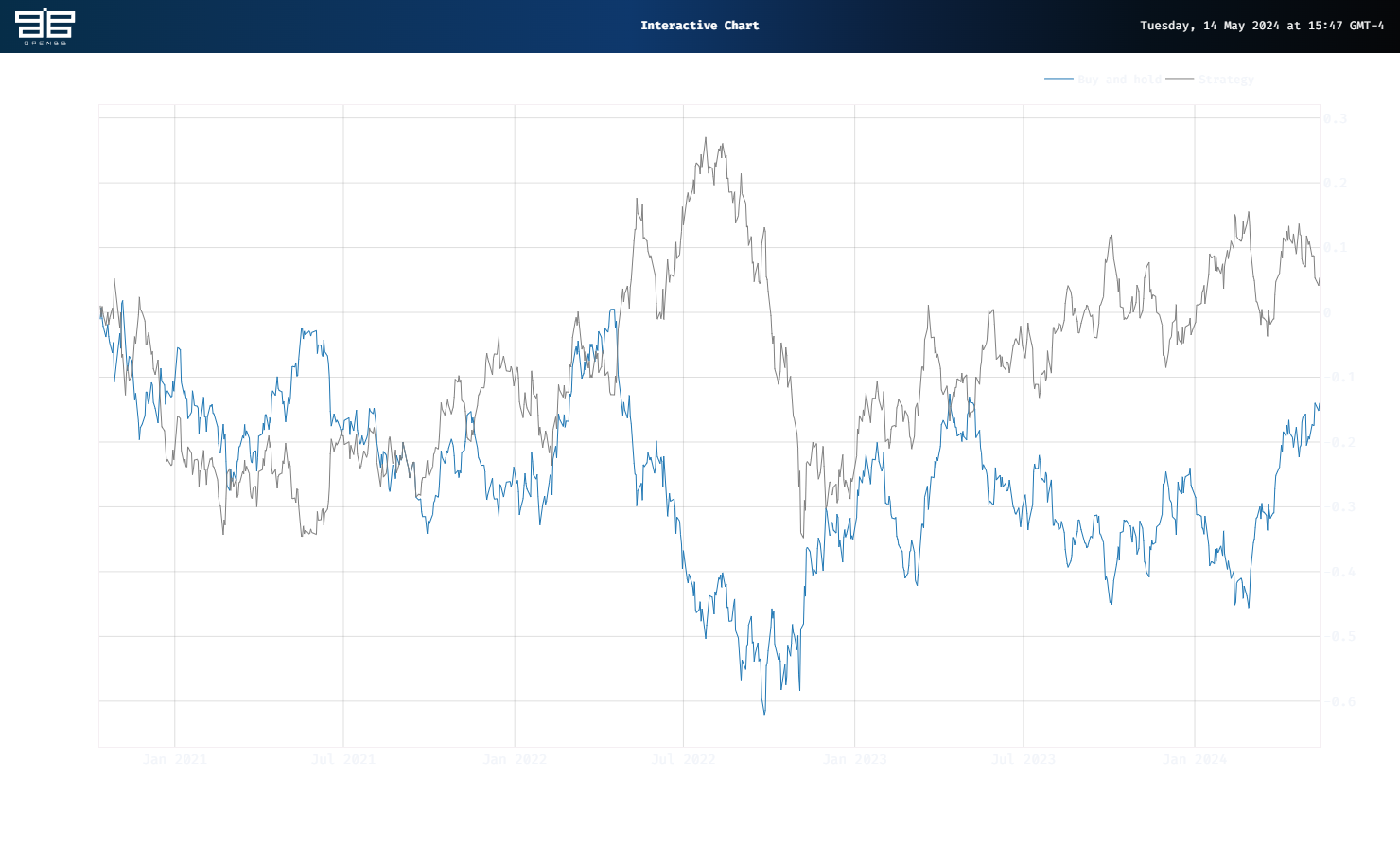
Not bad. The clustering regime strategy outperformed by almost 20 percentage points in the test period. Most of this is coming from the short side. Obviously, this is for illustrative purposes only, we’re not advocating owning or trading GDX anyway. The main point is we have a nice proof of concept for regime detection that we can iterate on in future posts with different ETFs. Stay tuned.
Here’s the code behind the results:
# Built using Python 3.10.19 and a virtual environment

# Install packages
from openbb import obb
import numpy as np
import pandas as pd
from hmmlearn.hmm import GaussianHMM
from sklearn.cluster import AgglomerativeClustering
from sklearn.mixture import GaussianMixture
import math
import warnings
warnings.filterwarnings('ignore')
import yfinance as yf

# Functions
def prepare_data_for_model_input(prices: pd.DataFrame, ma: int, instrument: str) -> pd.DataFrame, np.array:
    """
    Returns a dataframe with prices, moving average, and log returns as well as np.array of log returns
    """


    prices[f'{instrument}_ma'] = prices.rolling(ma).mean()
    prices[f'{instrument}_log_return'] = np.log(prices[f'{instrument}_ma']/prices[f'{instrument}_ma'].shift(1)).dropna()

    prices.dropna(inplace = True)
    prices_array = np.array([[q] for q in prices[f'{instrument}_log_return'].values])

    return prices, prices_array

class RegimeDetection:

    """
    Object to hold clustering, Gaussian Mixture or Hidden Markov Models
    """

  def get_regimes_hmm(self, input_data, params):
        hmm_model = self.initialise_model(GaussianHMM(), params).fit(input_data)
        return hmm_model

    def get_regimes_clustering(self, params):
        clustering =  self.initialise_model(AgglomerativeClustering(), params)
        return clustering

    def get_regimes_gmm(self, input_data, params):
        gmm = self.initialise_model(GaussianMixture(), params).fit(input_data)
        return gmm

    def initialise_model(self, model, params):
        for parameter, value in params.items():
            setattr(model, parameter, value)
        return model

def feed_forward_training(model: RegimeDetection, params: dict, prices: np.array, split_index: int, retrain_step: int, cluster: bool =False) -> list:
    """
    Returns list of regime states
    """

    # train/test split and initial model training
    init_train_data = prices[:split_index]
    test_data = prices[split_index:]
    if cluster:
        rd_model = model(params)
    else:
        rd_model = model(init_train_data, params)

    # predict the state of the next observation
    states_pred = []
    for i in range(math.ceil(len(test_data))):
        split_index += 1
        if cluster:
            preds = rd_model.fit_predict(prices[:split_index]).tolist()
        else:
            preds = rd_model.predict(prices[:split_index]).tolist()
        states_pred.append(preds[-1])

        # retrain the existing model
        if i % retrain_step == 0:
            if cluster:
                pass
            else:
                rd_model = model(prices[:split_index], params)

    return  states_pred

def get_strategy_df(prices_df: pd.DataFrame, split_idx: int, state_array: list, data_col: str, short: bool = False) -> pd.DataFrame:
    """
    Returns dataframe of prices and returns to buy and hold and strategy
    """

    prices_with_states = pd.DataFrame(prices_df[split_idx:][data_col])
    prices_with_states['state'] = state_array
    prices_with_states['ret'] = np.log(prices_with_states[data_col] / prices_with_states[data_col].shift(1)).dropna()
    prices_with_states['state'] = prices_with_states['state'].shift(1)
    prices_with_states.dropna(inplace = True)
    if short:
        prices_with_states['position'] = np.where(prices_with_states['state'] == 1, 1, -1)
    else:
        prices_with_states['position'] = np.where(prices_with_states['state'] == 1,1,0)
    prices_with_states['daily_hmm'] = prices_with_states['position'] * prices_with_states['ret']
    prices_with_states['Buy and hold'] = prices_with_states['ret'].cumsum()
    prices_with_states['Strategy'] = prices_with_states['daily_hmm'].cumsum()

    return prices_with_states

# Get data
symbol = "GDX"
data = obb.equity.price.historical(
    symbol=symbol,
    start_date="1999-01-01",
    provider="yfinance")
prices = pd.DataFrame(data.to_df()['close'])

prices, prices_array = prepare_data_for_model_input(prices, 10, 'close')

# If you want to graph the prices
# line_chart = data.charting.create_line_chart
# line_chart(
#     data=prices,
#     x=prices.index,
#     y="close",
#     title="GDX",
# )

# Create Regime and Backest
regime_detection = RegimeDetection()
model =  regime_detection.get_regimes_clustering
param_dict = {'gmm': {'n_components':2, 'covariance_type':"full", 'random_state':100, 'max_iter': 100000, 'n_init': 30,'init_params': 'kmeans', 'random_state':100},
              'clustering': {'n_clusters': 2, 'linkage': 'complete',  'affinity': 'manhattan', 'metric': 'manhattan', 'random_state':100},
              'hmm': {'n_components':2, 'covariance_type': 'full', 'random_state':100}
}
params = param_dict['clustering']
split_index = math.ceil(prices.shape[0] *.8)

# Generate regime
states = feed_forward_training(model, params, prices_array, split_index, 20, cluster=True)

# Add to price dataframe
prices['regime'] = np.nan
reg_idx = prices.columns.to_list().index('regime')
prices.iloc[split_index:, reg_idx] = np.array(states)
prices['regime_0'] = np.where(prices.regime == 0, prices.close, np.nan)
prices['regime_1'] = np.where(prices.regime == 1, prices.close, np.nan)

# Get Performance
prices_with_states = get_strategy_df(prices, split_index, states, 'close', short=True)

# Graph result
line_chart(
    data=prices_with_states,
    x=prices_with_states.index,
    y=['Buy and hold', 'Strategy'],
)