Not so soft softmax

Our last post examined the correspondence between a logistic regression and a simple neural network using a sigmoid activation function. The downside with such models is that they only produce binary outcomes. While we argued (not very forcefully) that if investing is about assessing the probability of achieving an attractive risk-adjusted return, then it makes sense to model investment decisions as probability functions. Moreover, most practitioners would probably prefer to know whether next month’s return is likely to be positive and how confident they should be in that prediction. They want to get direction right first. That’s binary.

But what about magnitude and relative performance? Enter multiclass logistic regression and neural networks with the softmax activation function. Typically multiclass (or multinomial) classifications are used to distinguish categories like Pekingese from Poodles, or Shih-tzus. With a bit of bucketing, one can do the same with continuous variables like stock returns. This may reduce noise somewhat, but also gets at the heart of investing: the shape of returns. Most folks who’ve been around the markets for a while know that returns are not normally distributed, particularly for stocks.¹ Sure, they’re fat-tailed and often negatively skewed. Discussed less frequently is that these returns also cluster around the mean. In other words, there are far more days of utter boredom, sheer terror, or unbearable ecstasy² than implied by the normal distribution.

While everyone wants to knock the ball out of the park and avoid the landmines, those events are difficult to forecast given their rarity even for the fat-tailed distribution. Sustained performance is likely to come from compounding in the solid, but hardly heroic area above the mean return near the one sigma boundary. These events are more frequent and also offer more data with which to work. Indeed, since 1970 almost 40% of the S&P 500’s daily returns fell into that area vs. the expectation of only 34% based on the normal distribution.

How would be go about classifying the probability of different returns? First, we’d bucket the returns according to some quantile and then run the regression or neural network on those buckets to get the predictions. Multiclass logistic regressions use the softmax function which looks like the following:

\[ Softmax(k, x_{1}, ..,, x_{n}): \Large\frac{e^{x_{k}}}{\sum_{i=1}^{n}e^{x_{i}}} \]

\[ f(k) = \begin{cases} 1 \text{ if } k = argmax(x_{1},...,x_{n}) \\ 0 \text{ othewise} \end{cases} \]

Here \(x_{k}\) is whatever combination of weights and biases with the independent variable that yields the maximum value for a particular class. Thus that value over the sum of all the exponentiated values yields the model’s likelihood for a particular category. How exactly does this happen? A multiclass logistic regression aggregates individual logistic regressions for the probability of each category with respect to all the other categories. Then it uses the fact that the probabilities must sum to one to yield the softmax function above. The intuition is relatively straightforward: how often do we see one class vs. all the rest based on some data? Check out the appendix for a (slightly!) more rigorous explanation.

Let’s get to our data, split it into the four quartiles for simplicity and then run a logistic regression on those categories. Recall we’re using the monthly return on the S&P500 as well as the return on the 10-month moving average vs. the one-month forward return, which we transform into the four buckets: below -1.9%, between -1.9% and 0.5%, between 0.5% and 3.6%, and above 3.6%. We’ll dub these returns with the following technical terms: Stinky, Poor, Mediocre, Good

Now we’ll run the regressions and present the confusion matrix as before.

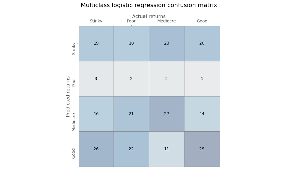
Whoa dude, is this some weird sudoku? Not really. Still, a four-by-four confusion matrix isn’t the easiest to read. Bear with us as we explain. The diagonal from the upper left to the lower right contains the true positives. The rows associated with each true positive are the false positives while the columns are the false negatives. The true negative is essentially all the other cells that don’t appear in either the row or the column for the particular category. So the true negative for the Stinky category would be the sum of the 3x3 matrix whose top left corner starts in the cell of the second row and second column.

Organizing the data this way is better than nothing, but it could be more insight provoking. We can see that the multiclass logistic regression is not that strong in the Poor category, but is much better in the Good category. Let’s compute the true positive and false positive rates along with the precision for each category, which we show in the table below.

Table 1: Logistic regression scores (%)

Outcome	TPR	FPR	Precision
Stinky	29.7	32.1	23.7
Poor	3.2	3.1	25.0
Mediocre	42.9	26.7	34.6
Good	45.3	31.1	33.0

Even with the refinement this still isn’t the easiest table to interpret. The model’s best true positive rate (TPR) performance is in the Good category, but it’s false positive rate (FPR) is also one of the highest. Shouldn’t we care about being really wrong? True, we don’t want to be consistently wrong. But we really don’t want to believe we’re going to generate a really good return and end up with a really Stinky one.

We’ll create a metric called the Really Wrong Rate (RWR) which will be the number of really wrong classifications over the total classifications the model made for that category. For example, for the Stinky outcome, the model got 19 correct (the top left box) but got 20 really wrong (the top right box). Thus its RWR is about 25% and its Precision to RWR is about 0.95. In other words, it’s getting more categories really wrong than correct.

What about the others? For the Good category, its RWR rate is almost 30% and its Precision to RWR is 1.12. That seems like a good edge. The model is really right about 12% more than it’s really wrong. However, when if you look at correctly identified categories plus incorrectly identified positive returns (the Good and Mediocre columns) relative to incorrectly identified categories with negative returns (the Stinky and Poor columns), the results are much worse: a ratio of about 0.83. Got that? Let’s move on to the neural network, before we get bogged down in confusion matrix navel gazing.

Unlike the linear regression or binary logistic regression, a simple neural network can’t approximate a multiclass logistic regression easily. Indeed, it takes a bit of wrangling to get something close, so we won’t bore you with all the iterations. We will show one or two just so you know how much effort we put in!

First, a single layer perceptron, with four output neurons, and a softmax activation function. We graph the model’s accuracy over 100 epochs along with logistic regression accuracy—the red dotted line—below.

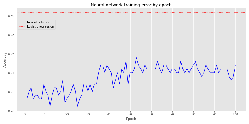
Not very inspiring. When we include a hidden layer with 20 neurons (an entirely arbitrary number!), but the same parameters as before, we get the following graph.

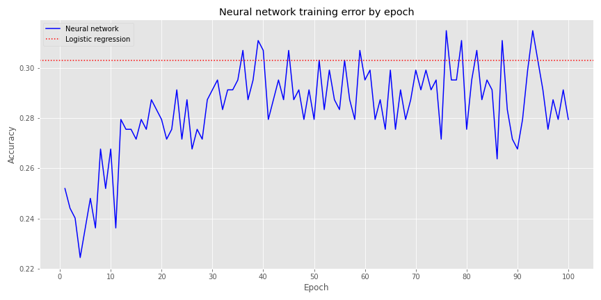
Definitely better. We see that around the 37th epoch, the NN’s accuracy converges with the logistic regression, but it does bounce around above and below that for the remaining epochs.

Let’s build a deeper NN, this time with three layers of 20 neurons each. For graphical purposes, the architecture of this NN looks like the following:

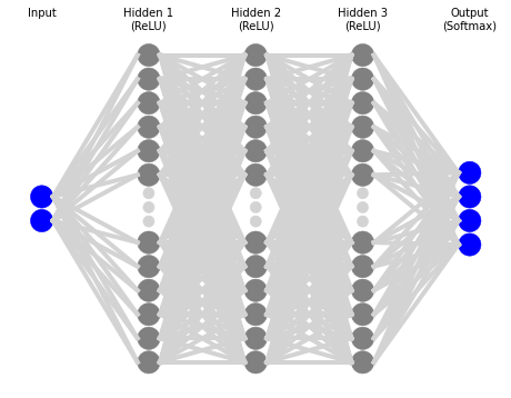
Plotting accuracy by epoch, gives us the next graph:

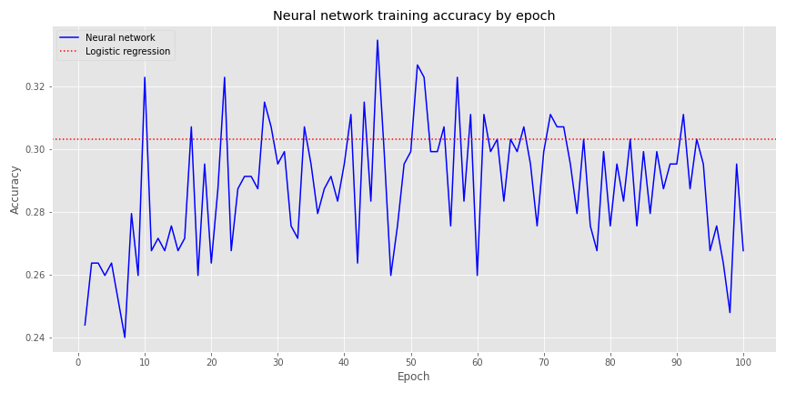
This denser NN achieves a better accuracy than the logistic regression sooner than the others, and it’s outperformance persists longer. Of course, even when it does perform worse, it isn’t that dramatic—about one or two percentage points.

We’ll stop the model at the first point that it converges with the logistic regression, which happens to the be the tenth epoch and create the confusion matrix is below.

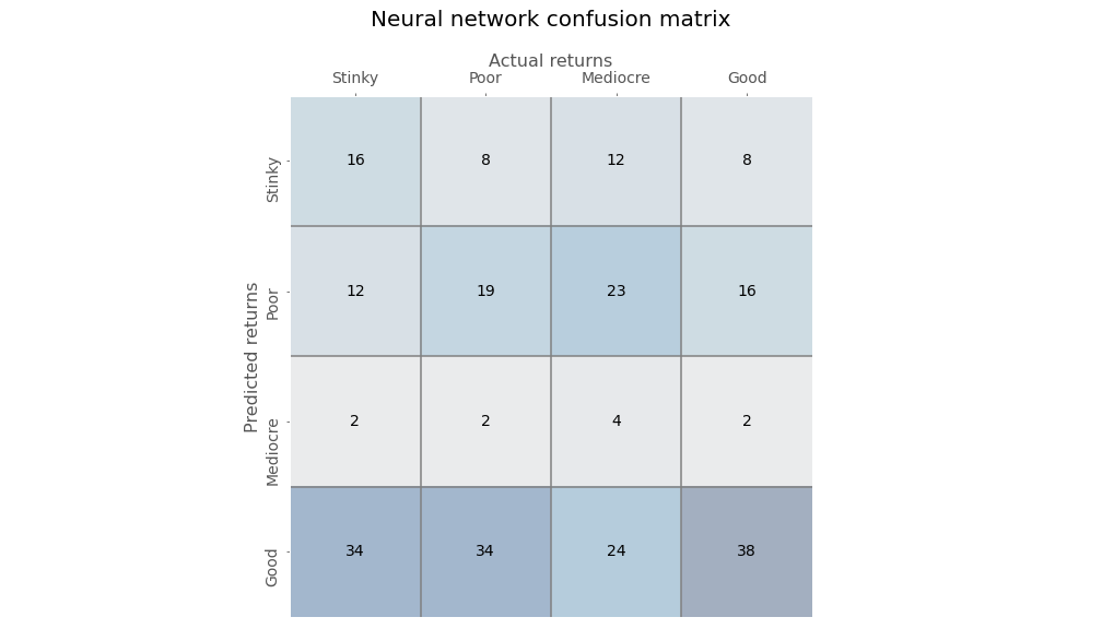
Again, a bit of struggle to discern much from this table, other than the model does not appear to predict Mediocre returns with much frequency even though they represent about 25% of the occurrences. Let’s look at some of the scores.

Table 2: Neural network scores (%)

Outcome	TPR	FPR	Precision
Stinky	25.0	14.7	36.4
Poor	30.2	26.7	27.1
Mediocre	6.3	3.1	40.0
Good	59.4	48.4	29.2

The NN model has a much better true positive rate (TPR) than the logistic regression for Good outcomes, but the false positive rate (FPR) is high too. While the NN model is worse than the regression model on Stinky outcomes, it’s FPR is less than half that of the regression. Interestingly, both models are poor at predicting one category: Poor outcomes for the regression model vs. Mediocre outcomes for the NN. We’re not sure why that would be the case.

The Stinky RWR is about 18% yielding a Precision to RWR ratio of 2 on the Stinky outcomes, much better than the logistic regressions ratio of 0.95. In other words, the NN is twice as likely to predict a Stinky outcome correctly than incorrectly predict a Good outcome as a Stinky one.

Should we favor the logistic regression over a NN with softmax activation? Hard to say. Accuracy results are similar, but we did have to play with the NN a lot more. More than accuracy, once you look under the hood, results diverge. The greater flexibility of the NN might help us tune a model to arrive at our desired true positive, false positive, and or really wrong rates. But that might come at the risk of overfitting. Moreover, it’s still unclear why both models picked one category as less likely even though the each category should have had an equal chance of occurring. We’d need to engage in more data analysis to figure out what we’re missing.

What are some other avenues we could explore? We could build denser neural networks. We could backtest the predictions to gauge performance. This would probably be done best using walk-forward analysis. Of course, a drawback with this is that few people were using neural networks to run trading algorithms during the 70s and 80s so the results could be spurious. That is, if people had been employing such algorithms, returns could have been a lot different. Another avenue is to change the bucketing mechanism so that we focus on the range of outcomes we’re most interested in or would be most likely to achieve high risk-adjusted returns.

We’ll leave those musings for now. Let us know what you’d like to read by sending an email to the address below. Want more on multiclass regressions and softmax functions? Or should we explore if neural networks can approximate decision trees and random forests? Let us know! Until then, have a look at the Appendix after the code. It walks through the link between logistic and softmax functions. And by all means, have a look at the code!

 Built using R 4.0.3, and Python 3.8.3

# [R]
# Load libraries
suppressPackageStartupMessages({
  library(tidyverse)
  library(tidyquant)
  library(reticulate)
})

# [Python]
# Load libraries
import warnings
warnings.filterwarnings('ignore')
import numpy as np
import pandas as pd
import statsmodels.api as sm
import matplotlib
import matplotlib.pyplot as plt
import os
os.environ['QT_QPA_PLATFORM_PLUGIN_PATH'] = 'C:/Users/user_name/Anaconda3/Library/plugins/platforms'

plt.style.use('ggplot')
plt.rcParams['figure.figsize'] = (12,6)

# Directory to save images

DIR = "your/image/directory" 

def save_fig_blog(fig_id, tight_layout=True, fig_extension="png", resolution=300):
    path = os.path.join(DIR, fig_id + "." + fig_extension)
    print("Saving figure", fig_id)
    if tight_layout:
        plt.tight_layout()
    plt.savefig(path, format=fig_extension, dip=resolution)
    

## Pull data and split
# See past posts for code
sp_mon = pd.read_pickle('sp_mon_tf_2.pkl')

data = sp_mon.dropna()

X_train = data.loc[:'1991', ['ret', '10ma_ret']]
y_train = data.loc[:'1991', '1_mon_ret'] 

X_valid = data.loc['1991':'2000', ['ret', '10ma_ret']]
y_valid = data.loc['1991':'2000', '1_mon_ret']

X_test = data.loc['2001':, ['ret', '10ma_ret']]
y_test = data.loc['2001':, '1_mon_ret']

y_train_trans = pd.qcut(y_train, 4, labels=[0, 1, 2, 3])

# Modest search for best solvers and regularization hyperparameters
from sklearn.linear_model import LogisticRegression

solvers = ['lbfgs', 'newton-cg', 'sag', 'saga']

for solver in solvers:
    log_reg = LogisticRegression(penalty='l2', solver = solver, multi_class='multinomial')
    log_reg.fit(X_train, y_train_trans)
    log_pred = log_reg.predict(X_train)
    print(log_reg.score(X_train, y_train_trans))
    
Cs = [10.0**-x for x in np.arange(-2,3)]

for c in Cs:
    log_reg = LogisticRegression(penalty='l2', multi_class='multinomial', C=c)
    log_reg.fit(X_train, y_train_trans)
    print(log_reg.score(X_train, y_train_trans))

log_reg = LogisticRegression(penalty='l2', multi_class='multinomial')
log_reg.fit(X_train, y_train_trans)
log_reg.score(X_train, y_train_trans)    
    
## Sigmoid on four classes
# Not shown
keras.backend.clear_session()
np.random.seed(42)
tf.random.set_seed(42)

y_train_cat = keras.utils.to_categorical(y_train_trans)

model = keras.models.Sequential([
    keras.layers.Dense(4, activation='sigmoid',input_shape = X_train.shape[1:])
])

model.compile(loss='binary_crossentropy', optimizer='sgd', metrics=['accuracy'])

history = model.fit(X_train, y_train_cat, epochs = 100)

## Softmax on four clases
keras.backend.clear_session()
np.random.seed(42)
tf.random.set_seed(42)

model = keras.models.Sequential([
    keras.layers.Dense(4, activation='softmax')
])

model.compile(loss='categorical_crossentropy', optimizer='sgd', metrics=['accuracy'])
history = model.fit(X_train, y_train_cat, epochs=100)

# Graph accuracy

log_score = log_reg.score(X_train, y_train_trans)
log_hist_df = pd.DataFrame(history.history)
log_hist_df.index = np.arange(1, len(log_hist_df)+1)
log_hist_df['accuracy'].plot(style='b-')
plt.axhline(log_score, color='red', ls = ':')
plt.xticks(np.arange(0,len(log_hist_df)+1, 10))
plt.xlabel('Epoch')
plt.ylabel('Accuracy')
plt.title("Neural network training error by epoch")
plt.legend(['Neural network', 'Logistic regression'], loc='upper left', bbox_to_anchor=(0.0, 0.9))
save_fig_blog('nn_vs_log_reg_tf3')
plt.show()

## Softmax with one hidden layer
keras.backend.clear_session()
np.random.seed(42)
tf.random.set_seed(42)

model = keras.models.Sequential([
    keras.layers.Dense(20, activation='relu', input_shape=X_train.shape[1:]),
    keras.layers.Dense(4, activation='softmax')
])

model.compile(loss='categorical_crossentropy', optimizer='sgd', metrics=['accuracy'])
history = model.fit(X_train, y_train_cat, epochs=100)

# Graph
log_score = log_reg.score(X_train, y_train_trans)
log_hist_df = pd.DataFrame(history.history)
log_hist_df.index = np.arange(1, len(log_hist_df)+1)
log_hist_df['accuracy'].plot(style='b-')
plt.axhline(log_score, color='red', ls = ':')
plt.xticks(np.arange(0,len(log_hist_df)+1, 10))
plt.xlabel('Epoch')
plt.ylabel('Accuracy')
plt.title("Neural network training error by epoch")
plt.legend(['Neural network', 'Logistic regression'], loc='upper left')
save_fig_blog('nn_vs_log_reg_2_tf3')
plt.show()

## Three hidden layer architecture
from nnv import NNV

layersList = [
    {"title":"Input\n", "units": 2, "color": "blue"},
    {"title":"Hidden 1\n(ReLU)", "units": 20},
    {"title":"Hidden 2\n(ReLU)", "units": 20},
    {"title":"Hidden 3\n(ReLU)", "units": 20},
    {"title":"Output\n(Softmax)", "units": 4,"color": "blue"},
]

NNV(layersList,max_num_nodes_visible=12, node_radius=8, font_size=10).render(save_to_file=DIR+"/nn_tf3.png")
plt.show()

## Softmax with three hidden layers
keras.backend.clear_session()
np.random.seed(42)
tf.random.set_seed(42)

model = keras.models.Sequential()
model.add(keras.layers.Dense(20, activation='relu', input_shape=X_train.shape[1:]))
for layer in range(2):
    model.add(keras.layers.Dense(20, activation='relu'))

model.add(keras.layers.Dense(4, activation='softmax'))
model.compile(loss='categorical_crossentropy', optimizer='sgd', metrics=['accuracy'])
history = model.fit(X_train, y_train_cat, epochs=100)


log_score = log_reg.score(X_train, y_train_trans)
log_hist_df = pd.DataFrame(history.history)
log_hist_df.index = np.arange(1, len(log_hist_df)+1)
log_hist_df['accuracy'].plot(style='b-')
plt.axhline(log_score, color='red', ls = ':')
plt.xticks(np.arange(0,len(log_hist_df)+1, 10))
plt.xlabel('Epoch')
plt.ylabel('Accuracy')
plt.title("Neural network training accuracy by epoch")
plt.legend(['Neural network', 'Logistic regression'], loc='upper left')
save_fig_blog('nn_vs_log_reg_3_tf3')
plt.show()

## Rerun stopping early
keras.backend.clear_session()
np.random.seed(42)
tf.random.set_seed(42)

model = keras.models.Sequential()
model.add(keras.layers.Dense(20, activation='relu', input_shape=X_train.shape[1:]))
for layer in range(2):
    model.add(keras.layers.Dense(20, activation='relu'))

model.add(keras.layers.Dense(4, activation='softmax'))

model.compile(loss='categorical_crossentropy', optimizer='sgd', metrics=['accuracy'])
history = model.fit(X_train, y_train_cat, epochs=10)

## Create confusion matrix table function
# Help from SO
# https://stackoverflow.com/questions/50666091/true-positive-rate-and-false-positive-rate-tpr-fpr-for-multi-class-data-in-py/50671617

from sklearn.metrics import confusion_matrix
# from sklearn.metrics import precision_score, recall_score, roc_curve

def conf_mat_table(predicted, actual, title = 'Logistic regression', save=False, save_title = None, print_metrics=False):
    
    conf_mat = confusion_matrix(y_true=predicted, y_pred=actual)

    fig, ax = plt.subplots(figsize=(14,8))
    ax.matshow(conf_mat, cmap=plt.cm.Blues, alpha=0.3)
    for i in range(conf_mat.shape[0]):
        for j in range(conf_mat.shape[1]):
            ax.text(x=j, y=i, s=conf_mat[i, j], fontsize=14, va='center', ha='center')

    ax.xaxis.set_ticks_position('top')
    ax.xaxis.set_label_position('top')
    ax.set_xticklabels(['','Stinky', 'Poor','Mediocre', 'Good'], fontsize=14)
    ax.set_yticklabels(['', 'Stinky', 'Poor', 'Mediocre', 'Good'], fontsize=14, rotation=90)
    ax.set_xlabel('Actual returns', fontsize=16)
    ax.set_ylabel('Predicted returns', fontsize=16)
    ax.tick_params(axis='both', which='major', pad=5)
    ax.set_title(title + ' confusion matrix', pad=40, fontsize=20)

    lines = [0.5, 1.5, 2.5]
    for line in lines:
        plt.axhline(line, color='grey')
        plt.axvline(line, color='grey')

    plt.grid(False)

    if save:
        save_fig_blog(save_title)
    plt.show()
    
    if print_metrics:
        FP = conf_mat.sum(axis=1) - np.diag(conf_mat)  
        FN = conf_mat.sum(axis=0) - np.diag(conf_mat)
        TP = np.diag(conf_mat)
        TN = conf_mat.sum() - (FP + FN + TP)
        
        # Add 1e-10 to prevent division by zero
        # True positive rate
        tpr = TP/(TP+FN+1e-10) 
        # Precision 
        precision = TP/(TP+FP+1e-10)
        # False positive rate
        fpr = FP/(FP+TN+1e-10)
                        
        print("")
        tab = pd.DataFrame(np.c_[['Stinky', 'Poor','Mediocre', 'Good'], tpr, fpr, precision], 
                           columns = ['Outcome', 'TPR', 'FPR', 'Precision']).set_index("Outcome")

        tab = tab.apply(pd.to_numeric)    
    
        return tab, conf_mat
    

## Predictions
log_pred = log_reg.predict(X_train)
nn = model.predict(X_train)
nn_pred = np.argmax(nn, axis=1)

## Logistic regression table

tab1, conf_mat1 = conf_mat_table(log_pred, y_train_trans, save=False, title="Multiclass logistic regression", 
                                 print_metrics=True, save_title='log_reg_conf_mat_1_tf3')

# Save to csv for blog
dir1 = "your/wd"
folder = "/your_folder/"
tab1.to_csv(dir1+folder+'tab1_tf3.csv')

conf_mat1 = pd.DataFrame(data = conf_mat1, index=pd.Series(['Stinky', 'Poor','Mediocre', 'Good'], name='Outcome'), 
             columns=['Stinky', 'Poor','Mediocre', 'Good'])
conf_mat1.to_csv(dir1+folder+'/conf_mat1_tf3.csv')

# [R]
# Rmarkdown table
# Asssumes we're in the directory to which we saved all those csvs.
tab1 <- read_csv('tab1_tf3.csv')

tab1 %>% 
  mutate_at(vars("TPR", "FPR", "Precision"), 
            function(x) format(round(x,3)*100,nsmallest=0)) %>% 
  knitr::kable(caption = "Logistic regression scores (%)")

conf_mat1 <- read_csv('conf_mat1_tf3.csv')

stinky_rwr <- as.numeric(conf_mat1[1,5]/sum(conf_mat1[1,2:5]))
good_rwr <- as.numeric(conf_mat1[4,2]/sum(conf_mat1[4,2:5]))

stinky_prec <- as.numeric(tab1[1,4])
good_prec <- as.numeric(tab1[4,4])
good_2_Stinky <- (sum(conf_mat1[4,4:5])/sum(conf_mat1[4,2:3]))

# [Python]
## Neutral network table
tab2, conf_mat2 = conf_mat_table(nn_pred, y_train_trans, title="Neural network", save=False, print_metrics=True, save_title='nn_conf_mat_1_tf3')

# Save to csv for blog
tab2.to_csv(dir1+folder+'/tab2_tf3.csv')

conf_mat2 = pd.DataFrame(data = conf_mat2, index=pd.Series(['Stinky', 'Poor','Mediocre', 'Good'], name='Outcome'), 
             columns=['Stinky', 'Poor','Mediocre', 'Good'])
conf_mat2.to_csv(dir1[:-13]+'/conf_mat2_tf3.csv')
conf_mat2.to_csv(dir1+folder+'/conf_mat2_tf3.csv')


# [R]
# Rmarkdown table
# Neural network
# Asssumes we're in the directory to which we saved all those csvs.
tab2 <- read_csv('tab2_tf3.csv')

tab2 %>% 
  mutate_at(vars("TPR", "FPR", "Precision"), function(x) format(round(x,3)*100,nsmallest=0)) %>% 
  knitr::kable(caption = "Neural network scores")

conf_mat2 <- read_csv('conf_mat2_tf3.csv')

stinky_rwr1 <- as.numeric(conf_mat2[1,5]/sum(conf_mat2[1,2:5]))
good_rwr1 <- as.numeric(conf_mat2[4,2]/sum(conf_mat2[4,2:5]))
stinky_prec1 <- as.numeric(tab2[1,4])
good_prec1 <- as.numeric(tab2[4,4])
good_2_Stinky1 <- (sum(conf_mat2[4,4:5])/sum(conf_mat2[4,2:3]))