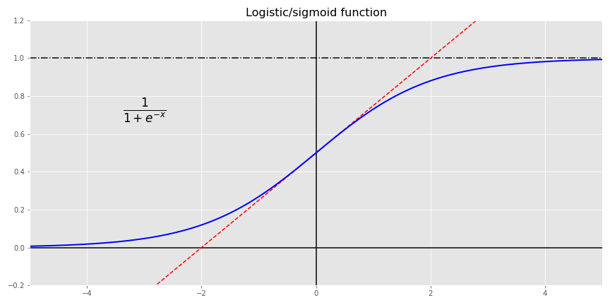
Activate sigmoid!

In our last post, we introduced neural networks and formulated some of the questions we want to explore over this series. We explained the underlying architecture, the basics of the algorithm, and showed how a simple neural network could approximate the results and parameters of a linear regression. In this post, we’ll show how a neural network can also approximate a logistic regression and extend our toy example.

What’s the motivation behind showing the link with logistic regression? If one accepts that investing is about assessing the probability of achieving an attractive risk-adjusted return, then it makes sense to model investment decisions as probability functions. The logistic function returns a binary probability. Indeed, the New York Fed publishes a recession probability model that predicts the likelihood of a recession in the next twelve months, using a function similar to a logistic regression. A recent search of Google scholar returned over 50,000 results for the terms stock price prediction and logistic regression.

Besides using a model that more closely approximates the decision process, another reason to use a logistic regression has to do with the structure of price and return data. It’s noisy. A linear regression may interpret that noise as meaningful, yielding too precise of an output. Is it more important to know whether next month’s return is likely to be 5.352% or 5.438%? Probably not. Rather, most practitioners would prefer to know whether next month’s return is likely to be positive and how confident they can be in that prediction. Magnitude and relative performance are important too. But you’ve got to get direction right first. Feel free to disagree.

Thus modeling potentially predictive features as a probability is likely to be more intuitive in many cases. How this works in practice is the following. The potentially explanatory variables are regressed to find the the log-odds (\(log(\frac{p}{1-p})\)) for some event. Then by the beauty of math, one transforms the log-odds into the logistic function (\(\frac{1}{1 + e^{-x}}\)) which yields a value between zero and one, the probability of the outcome. Don’t get too bogged down in why log-odds are used other than to note that it makes the math more tractable. See the Appendix after the code for more detail and how to derive the logistic function from the log-odds.

It just so happens that the logistic function, or sigmoid function as it is sometimes called¹ is one of the activation functions used in neural networks. Recall, the \(\phi\) from the last post that is used to transform the aggregated weights and biases from a layer of neurons into the desired output form? Sigmoid is one of those activation functions!²

How does this all relate to investing? Let’s go back to our data: the S&P 500 and the 10-month moving average. Given the month-end closing price and the moving average, what’s the probability the index will be positive in the next month? If you’re an Efficient Market acolyte, your answer is it’s random: could be positive, could be negative; but you’ve got no better than a coin flip’s chance in predicting what it will be. In many cases that’s true, but let’s look at the data to illustrate our investigation.

We’ll transform all of our data into returns and convert next month’s return into a [1,0] output to signify a positive or not positive return. Given that we’re dealing with probabilities, we’ll convert the results into a confusion matrix to see how well the logistic regression model performs. The table gives the number of outcomes in which the model predicted a positive or negative return in the next month vs. an actual positive or negative return.

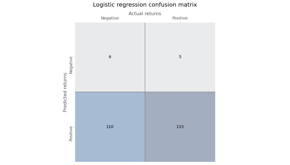
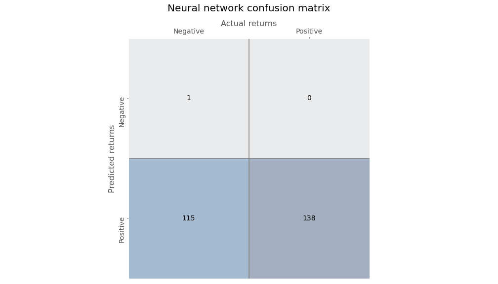
Gazing at the figures in the second column, one can see that the logistic regression has an exceedingly high recall or true positive rate. In other words, of all the positive outcomes (the second column, or 133 + 5), how many did the model accurately predict (the lower right hand box, or 133)? Before, we discuss this and other useful metrics, we’ll run the neural network (NN) and look at its confusion matrix. This NN is a simple one just like before: no hidden layer, but with a sigmoid activation function.

Ok. Let’s compare the results.

Model	Recall/True positve rate	False positve rate	Precision
Regression	96.4%	94.8%	54.7%
Neural network	100.0%	99.1%	54.5%

Wow! Look at that true positive rate. The logistic regression was awesome, but the neural network was flawless. Wait a second, look at the false positive rate. Atrocious! The false positive rate is essentially the flipside of the true negative rate, and corresponds to the first column in the tables above. It answers the question, out of all the negative outcomes, how many did model predict incorrectly? In this case, almost all of them! That doesn’t bode well for a good investing model. You don’t want to follow recommendations that tell you to get long when the opposite is likely happen, unless the magnitude of the return when the recommendations are right meaningfully offsets the times when they’re wrong.

Let’s discuss precision, or how often the model was correct when it predicted a positive return. Both models are slightly better than a coin flip, with a precision of around 55%. While that might seem pretty darn good in market lore—lots of traders say you only need to be right a bit more than 50% of the time to generate good returns—is it good enough? In our training set, we found that returns were positive 54.3% of the time. Naively predicting only positive returns wouldn’t be much worse than the models without getting a headache trying to figure out all the math. Clearly, the models don’t provide much more insight than using some rough averages.

Of course, our point is not to find the best predictive model; rather, to show the correspondence between a logistic regression and a simple neural network with a sigmoid activation function. A better model would seek to lower the false positive rate. But, as you data science/machine learning gurus know, there’s a trade-off between the true positive and false positive rate. One way to lower the false positive rate is with thresholding. That is, require a higher probability to predict a positive outcome. For example, since we know that returns are positive 54% of the time, we could require the logistic regression model to predict a positive return only if the regression probabilities exceed that number. In effect, only when the model is more confident than the base rate will we allow it to predict a positive return.

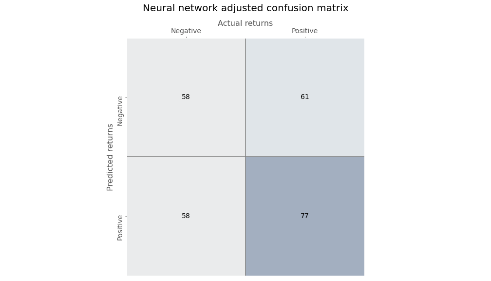
Employing thresholding yields the following confusion matrix.

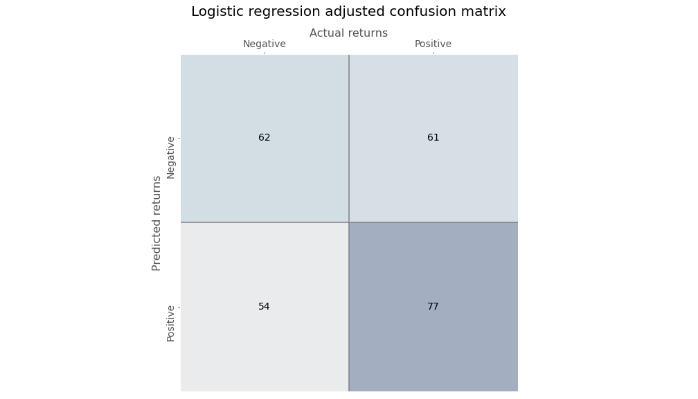
Just eyeballing the numbers shows a more balanced output.

Thresholding for the NN is a little trickier. To explain why, we need to delve into what each algorithm is doing. The logistic regression calculates the coefficients of the independent variables to get as close as possible to the observed log-odds. Then for an observed input, it plugs the numbers into the equation, calculates the log-odds, transforms that into a probability, and if the probability is above 50%, outputs a \(1\) for a positive outcome.

The neural network, on the other hand, takes the data, applies weights and a bias to that data, and then puts that result through an activation function. It assesses the quality of that by calculating a loss function of the actual vs. predicted values and then tries to minimize the loss by iteratively tweaking the weights and bias with respect to the loss function.

The methods practitioners use to generate a logistic regression³ is iterative like the NN. But the NN is trying to minimize whatever loss function⁴ you give it, while the logistic regression is trying maximize the likelihood of producing the observed probability. Same, same, but different.

If this all seems a bit arcane, no worries. Just know that since one is minimizing the loss, while the other is maximizing the odds, the probabilities won’t necessarily be the same even if the predictions are pretty close. Ultimately, we can get to a similar result as the logistic regression by changing the threshold a little bit,⁵ as shown below.

Now that we’ve established that we can arrive at similar predictions for both the logistic regression and the NN, let’s compare the two models. For a given input, what probability does each model ascribe to a positive outcome? As we’ve already intimated, the probabilities are not at all the same. In the chart below, we graph the logistic regression probabilities against the NN and include a \(45^o\) line as a way to compare relative “confidence”.

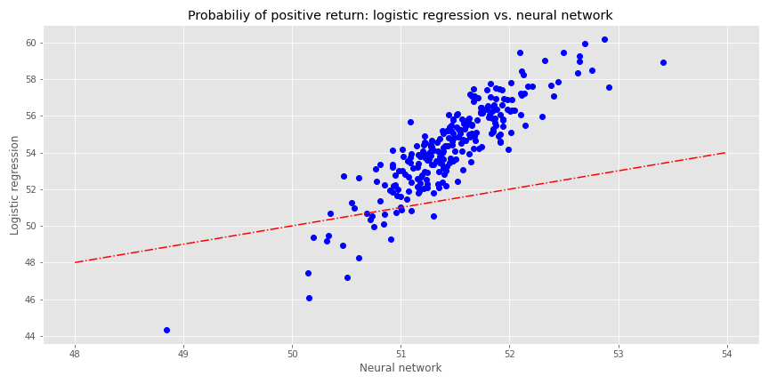The logistic regression is decidedly above the line, but more spread out than the NN, indicating more confidence but less precision in its results. In fact, the logistic regression probabilities are higher than the NN almost 90% of the time. Why should that be the case when the predictions are quite similar? Part of this is likely due to the activation function. The sigmoid function tends to push values toward 50%, so we can see most of the NN’s probabilities lie close to that value. The logistic regression pushes the regression coefficients to get as close to the log-odds, which, based on the positive return frequency, is a probability of around 54%. As one can see on the graph, 54% is the mid-range for the logistic regression. Critically, the graph shows why thresholding needs to be slightly lower for the NN to obtain similar predictions as the regression.

Does this mean that we should trust a NN more than a logistic regression? From a risk management perspective, it is perhaps better to employ a model that is relatively more uncertain when the predictions themselves aren’t that great in the first place. But this is probably overstated, as the differences in results seem to be heavily influenced by the idiosyncrasies of each model. Broadly speaking, should we ascribe more or less confidence or precision when the differentials are usually around five percentage points or less? Probably not. And even talking about confidence might be confusing a metaphor with reality. Who says you can’t anthropomorphize math!

Where does this leave us? We’ve shown the correspondence between a logistic regression and a neural network. Both can arrive at similar predictions even if they get there using different methods. In our example, both models were pretty abysmal. But we weren’t trying to build the perfect model. Although we only discussed binary events, both models can handle multi-class ones, albeit using different methods.

At this early stage, it’s still not clear that neural networks produce better results than traditional methods. They were both equally bad in this post! We can say, however, that neural networks have the flexibility to approximate some of the traditional regression techniques and we have yet to tap their full potential. Next time we’ll explore multi-class events and employ a deeper neural network. Until then, here’s the code:

 Built using R 4.0.3, and Python 3.8.3

# [R]
# Load libraries
suppressPackageStartupMessages({
  library(tidyverse)
  library(tidyquant)
  library(reticulate)
})

# [Python]
# Load libraries
import warnings
warnings.filterwarnings('ignore')
import numpy as np
import pandas as pd
import statsmodels.api as sm
import matplotlib
import matplotlib.pyplot as plt
import os
os.environ['QT_QPA_PLATFORM_PLUGIN_PATH'] = 'C:/Users/user_name/Anaconda3/Library/plugins/platforms'

plt.style.use('ggplot')
plt.rcParams['figure.figsize'] = (12,6)

# Directory to save images
# Most of the graphs are now imported as png. We've explained why in some cases that was necessary due to the way reticulate plays with Python. But we've also found that if we don't use pngs, the images don't get imported into the emails that go to subscribers. 

DIR = "your/image/directory" 

def save_fig_blog(fig_id, tight_layout=True, fig_extension="png", resolution=300):
    path = os.path.join(DIR, fig_id + "." + fig_extension)
    print("Saving figure", fig_id)
    if tight_layout:
        plt.tight_layout()
    plt.savefig(path, format=fig_extension, dip=resolution)
    
## Plot sigmoid activation function
## Note: code developed from Hands-on Machine learning with Scikit-Learn, Keras, and Tensorflow
## Github source: https://github.com/ageron/handson-ml2/blob/master/11_training_deep_neural_networks.ipynb
    
def logit(x):
    return 1/(1+np.exp(-x))

x = np.linspace(-5, 5, 200)

plt.plot([-5, 5], [0, 0], 'k-')
plt.plot([-5, 5], [1, 1], 'k--')
plt.plot([0, 0], [-0.2, 1.2], 'k-')
plt.plot([-5, 5], [-3/4, 7/4], 'r--')
plt.plot(x, logit(x), "b-", linewidth=2)
plt.annotate('The function: $\\frac{1}{1+e^{-x}}$', xy=(-4,0.7), fontsize=20)
plt.grid(True)
plt.title("Sigmoid activation function", fontsize=16)
plt.axis([-5, 5, -0.2, 1.2])

save_fig_blog("sig_func_tf2")
plt.show()
    

## Pull S&P data and process
start = '1970-01-01'
end = '2020-12-31'

sp = dr.DataReader('^GSPC', 'yahoo', start, end)

sp_mon = pd.DataFrame(sp['Adj Close'].resample('M').last())
sp_mon['10ma'] = sp_mon['Adj Close'].rolling(10).mean()
sp_mon.columns = ['close', '10ma']
sp_mon = sp_mon.rename(index = {'Date':'date'})

sp_mon['ret']= sp_mon['close'].pct_change()


# Add month forward
sp_mon['1_mon'] = sp_mon['close'].shift(-1)

## Create train, valid, test split
data = sp_mon.dropna()

X_train = data.loc[:'1991', ['ret', '10ma_ret']]
y_train = data.loc[:'1991', '1_mon_ret'] 

X_valid = data.loc['1991':'2000', ['ret', '10ma_ret']]
y_valid = data.loc['1991':'2000', '1_mon_ret']

X_test = data.loc['2001':, ['ret', '10ma_ret']]
y_test = data.loc['2001':, '1_mon_ret']

y_train_log, y_valid_log, y_test_log = (y_train > 0).astype('int'), (y_valid > 0).astype('int'), (y_test > 0).astype('int')

## Run logistic regression
from sklearn.linear_model import LogisticRegression

log_reg = LogisticRegression(penalty='none')
log_reg.fit(X_train, y_train_log)
log_pred = log_reg.predict(X_train)
log_mse = np.mean((log_pred - y_train_log)**2)

## Create Neural network and run
keras.backend.clear_session()
np.random.seed(42)
tf.random.set_seed(42)

log_nn = keras.models.Sequential([
    keras.layers.Dense(1, activation='sigmoid',input_shape = X_train.shape[1:])
])

log_nn.compile(loss='binary_crossentropy', optimizer='sgd')

log_hist = log_nn.fit(X_train, y_train_log, epochs = 20)

## Create confusion matrix function
from sklearn.metrics import confusion_matrix
from sklearn.metrics import precision_score, recall_score, roc_curve

def conf_mat_table(predicted, actual, title = 'Logistic regression', save=False, save_title = None, print_metrics=True):
    
    conf_mat = confusion_matrix(y_true=predicted, y_pred=actual)

    fig, ax = plt.subplots(figsize=(14,8))
    ax.matshow(conf_mat, cmap=plt.cm.Blues, alpha=0.3)
    for i in range(conf_mat.shape[0]):
        for j in range(conf_mat.shape[1]):
            ax.text(x=j, y=i, s=conf_mat[i, j], va='center', ha='center')

    ax.xaxis.set_ticks_position('top')
    ax.xaxis.set_label_position('top')
    ax.set_xticklabels(['','Negative', 'Positive'])
    ax.set_yticklabels(['', 'Negative', 'Positive'], rotation=90)
    ax.set_xlabel('Actual returns', fontsize=12)
    ax.set_ylabel('Predicted returns', fontsize=12)

    plt.axhline(0.5, color='grey')
    plt.axvline(0.5, color='grey')
    plt.grid(False)
    plt.title(title + ' confusion matrx', pad=30, fontsize = 14)

    if save:
        save_fig_blog(save_title)
    plt.show()
    
    if print_metrics:
        fpr, tpr, _ = roc_curve(actual, predicted)
        precision = precision_score(actual, predicted)
        recall = recall_score(actual, predicted)
        
        print("")
        print(f'Precision = {precision*100:0.1f}%')
        print(f'Recall = {recall*100:0.1f}%')
        print(f'True Positive Rate = {tpr[1]*100:0.1f}%')
        print(f'False Positive Rate = {fpr[1]*100:0.1f}%')

# confusion matrix for logistic regression            
conf_mat_table(log_pred, y_train_log, save=True, save_title = 'log_reg_conf_tab_1_tf2')

# confusion matrix for NN
nn_pred = (log_nn.predict(X_train) >= y_train_log.mean()).astype('int').flatten()
conf_mat_table(nn_pred, y_train_log, title='Neural network', save=True, save_title = 'nn_conf_tab_1_tf2')

# confusion matrix for logistic regression with thresholding
conf_mat_table(log_pred_adj, y_train_log, title='Logistic regression adjusted', save=True, save_title = 'log_reg_adj_conf_tab_1_tf2')

# confusion matrix for NN with thresholding
nn_pred = (log_nn.predict(X_train) > 0.5125).astype('int').flatten()
conf_mat_table(nn_pred, y_train_log, "Neural network adjusted", save=True, save_title='nn_adj_conf_tab_1_tf2')

# Graph logistic regression vs NN probabilities
log_prob = log_reg.predict_proba(X_train)[:,1]*100
nn_prob = log_nn.predict(X_train)*100
xs = np.linspace(48, 54,50)
ys = xs

plt.figure()
plt.plot(nn_prob, log_prob, 'bo')
plt.plot(xs, ys, 'r-.')
# plt.xlim([0.44,0.62])
# plt.ylim([0.44,0.62])
plt.ylabel('Logistic regression')
plt.xlabel('Neural network')
plt.title("Probabiliy of positive return: logistic regression vs. neural network")
save_fig_blog('log_reg_vs_nn_tf2')
plt.show()