What do machines know about the yield curve?

A recession a year from now?

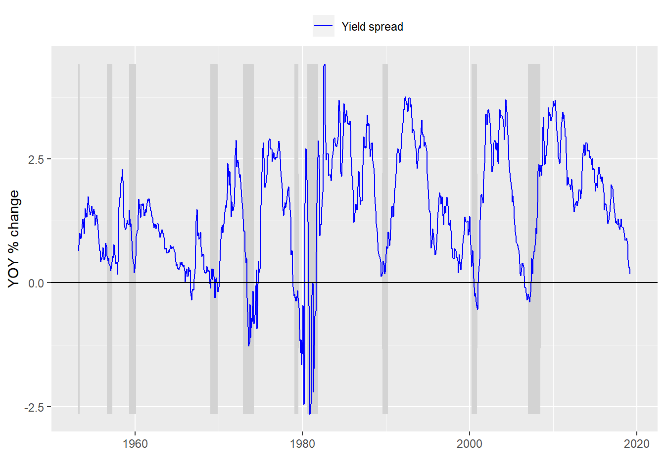
We can dispense with much of the discussion about building the model since we’ve covered that in other posts. Here we’lll just present the data and move on to a machine learning model. Here’s a chart of the yield curve with recessions adjusted for the 12-month look forward.

Now we create a model based on that look forward period and present the confusion matrix

Predicted/Actual	No recession	Recession
No recession	676	86
Recession	13	17

And here are the usual metrics:

With the usual metrics:

• Accuracy: 88%
• Specificity: 17%
• False positive rate: 83%

The model’s accuracy is about the same as the 6-month look forward. While the specification is modestly better. But this comes with the trade-off of a higher false positive rate. But at a very low rate of 2% the trade-off is probably worth it.

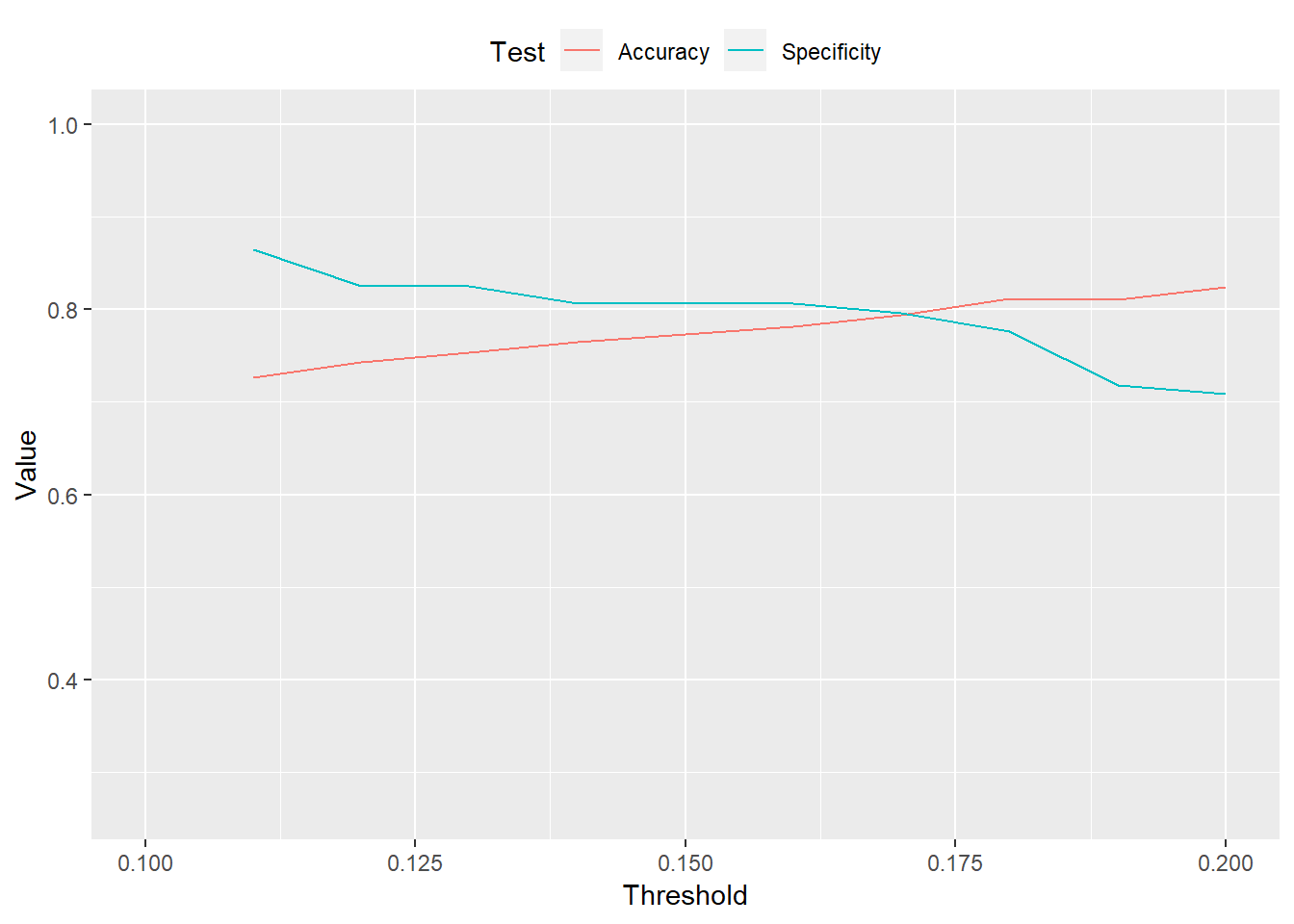
Now we look at varying thresholds for the recession prediction

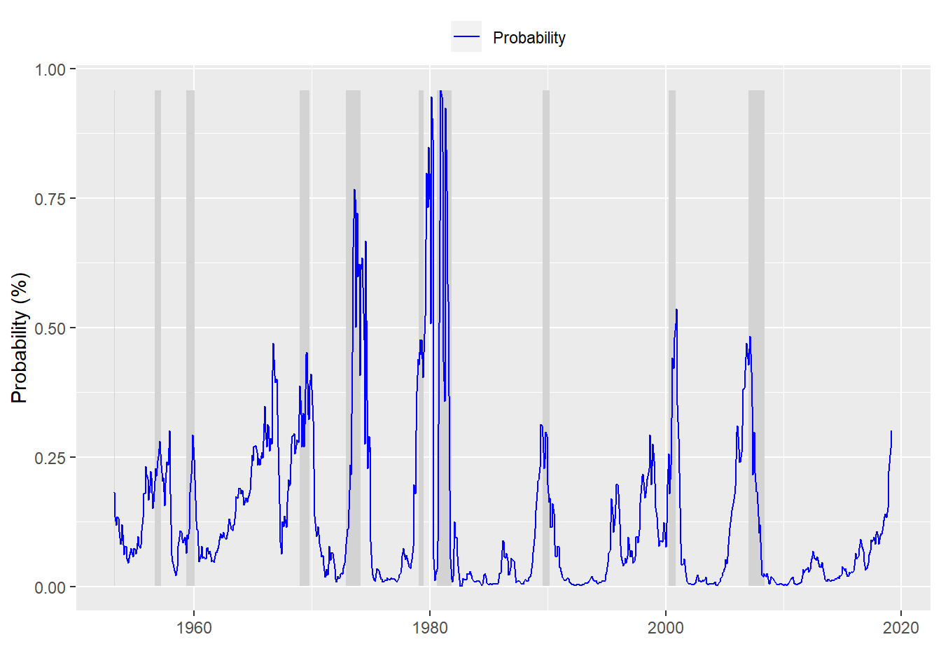
And for those interested, here is a graph of the probabilities of a recession based on the 12-month look forward. Interestingly, even when the model is in the midst of a recession, it predicts the probability of a recession often less than 50%.

This is all well and good (if a little academic). The main problem is that we’ve bulit a model on all the available data. How do we know this model will work on new data? For that we need to use some relatively straightforward machine learning techniques. We’ll split the data into training and test sets. Build the model on the training set and then test its predictive ability on the test set.

We need to consider a couple of issues before we move forward. Where do we split the data? And how reliable should we consider these results since there have only been about 10 recessions in the last 65 years. The second issue is a bit thornier and will shelve that for the next post.

On the first issue, we don’t have a good analytical answer as to where we should split the data. We can run the model on different train/test splits, which we can try in later episodes. But for now we’ll use 1999 as the cut-off.

Predicted/Actual	No recession	Recession
No recession	216	26
Recession	1	0

The usual metrics:

• Accuracy: 89%
• Specificity: 0%
• False positive rate: 100%

Great…zero ability to predict a recession correctly. But we’re using the 50% threshold as before. If we use a 15% threshold, in line with the recession base rate we generate the following results:

Predicted/Actual	No recession	Recession
No recession	192	8
Recession	25	18

Revised metrics:

• Accuracy: 86%
• Specificity: 69%
• False positive rate: 31%

This isn’t bad. The accuracy remains high relative to prior models, but specificity increases significantly. Of course, that comes at the cost of a much higher false positive rate. But should we be worried about the effects of such a high false positive rate? That will have to wait.

Here’s the code behind everything above:

# Load package
library(tidyquant)

# Load data
df <- readRDS("yield_curve.rds")

# Process data
df_12 <- df %>% mutate(usrec = lead(usrec, 12, default = 0))

# Plot data
df_12 %>% ggplot(aes(x = date)) +
  geom_ribbon(aes(ymin = usrec*min(time_spread), ymax = usrec*max(time_spread)), fill = "lightgrey") +
  geom_line(aes(y = time_spread, color = "Yield spread")) +
  scale_colour_manual("", 
                      breaks = c("Yield spread"),
                      values = c("blue")) +
  ylab("YOY % change") + xlab("") + ylim(c(min(df_12$time_spread), max(df_12$time_spread))) +
  geom_hline(yintercept = 0, color = "black") +
  theme(legend.position = "top", legend.box.spacing = unit(0.05, "cm"))

# Create model
model_12 <- glm(usrec ~ time_spread, df_12, family = binomial)

# Predict on test set
pred_12 <- predict(model_12, df_12, type = "response")
  
# Confusion matrix
probs_12 <- rep(0,nrow(df_12))
probs_12[pred_12 > 0.5] <- 1
tab <- table(Predicted = probs_12, Actual = df_12$usrec)
rownames(tab) <- c("No recession", "Recession")
colnames(tab) <- c("No recession", "Recession")
library(printr)
tab

# Build specification function
spec_func <- function(threshold, df){
  probs <- pred_12 > threshold
  tab <- table(probs, df$usrec)
  if(nrow(tab) == 1){
    return(0)
  }else{
    return(tab[2,2]/(tab[2,2] + tab[1,2]))
  }
}

# Build accuracy function
acc_func <- function(threshold, df){
  probs <- pred_12 > threshold
  tab <- table(probs, df$usrec)
  if(nrow(tab) == 1){
    return(tab[1,1]/sum(tab))
  }else{
    return((tab[2,2] + tab[1,1])/sum(tab))
  }
}

# Run specification
spec_12 <- c()
for(i in 1:20){
  spec_12[i] <- spec_func(i*.01, df_12)
}

# Run accuracy
acc_12 <- c()
for(i in 1:20){
  acc_12[i] <- acc_func(i*.01, df_12)
}

# Create data frame, tidy, and graph
acc_spec_12 <- data.frame(Threshold = seq(0.01, 0.20, 0.01), Accuracy = acc_12, Specificity = spec_12)
acc_spec_12 <- acc_spec_12 %>% gather(Test, Value, -Threshold)
acc_spec_12 %>% ggplot(aes(Threshold, Value, color = Test)) + 
  geom_line() + 
  xlim(c(0.1,0.2)) +  
  theme(legend.position = "top", legend.box.spacing = unit(0.05, "cm"))

# Plot probabilities
df_12 %>% 
  mutate(prob = pred_12) %>%
  ggplot(aes(x = date)) +
  geom_ribbon(aes(ymin = usrec*min(prob), ymax = usrec*max(prob)), fill = "lightgrey") +
  geom_line(aes(y = prob, color = "Probability")) +
  scale_colour_manual("", 
                      breaks = c("Probability"),
                      values = c("blue")) +
  ylab("Probability (%)") + xlab("") + ylim(c(min(pred_12), max(pred_12))) +
  theme(legend.position = "top", legend.box.spacing = unit(0.05, "cm"))

# Create train and test sets
start_date_train <- "1953-04-01"
end_date_train <- "1998-12-31"
train <- df_12 %>% filter(date >= start_date_train, date <= end_date_train)
test <- df_12 %>% filter(date > end_date_train)
  
# Fit model on train set
train_fit <- glm(usrec ~ time_spread, train, family = binomial)
  
# Predict on test set
pred_test <- predict(train_fit, test, type = "response")
  
# Confusion matrix
probs_test <- rep(0,nrow(test))
probs_test[pred_test > 0.5] <- 1
tab_test <- table(Predicted = probs_test, Actual = test$usrec)
rownames(tab_test) <- c("No recession", "Recession")
colnames(tab_test) <- c("No recession", "Recession")
tab_test

# Confusion matrix
probs_new <- rep(0,nrow(test))
probs_new[pred_test > 0.15] <- 1
tab_new <- table(Predicted = probs_new, Actual = test$usrec)
rownames(tab_new) <- c("No recession", "Recession")
colnames(tab_new) <- c("No recession", "Recession")
tab_new