My strategy beats yours!
Don’t hold your breath. We’re taking a break from our deep dive into diversification. We know how you couldn’t wait for the next installment. But we thought we should revisit our previous post on investing strategies to mix things up a bit. Recall we investigated whether employing a 200-day moving average tactical allocation would improve our risk-return proflie vs. simply holding a large cap index like the S&P500.
What we learned when we calculated rolling twenty-year cumulative returns was that the moving average strategy outperformed the S&P 500 76% of the time. However, that performance was mainly front-end loaded. Since 1990, the moving average strategy only outperformed 59% of the time. These results led us to ask the following questions:
Does the tactical allocation allow us to hit our long-term return goal with a higher probability than simply investing in the index?
If it does, is it worth the extra effort to execute the strategy?
The second question delves more into the field of behavioral finance, which is much tougher to quantify. We’ll shelve that one momentarily. To answer the first question, we should of course look at the historical record a little more deeply and then try and simulate multiple scenarios to see what the cut-offs might be.
Show me the history
Let’s first look at the historical results. We calculate the yearly cumulative return of the moving average strategy and the S&P500 and then graph the outperformance of the strategy.
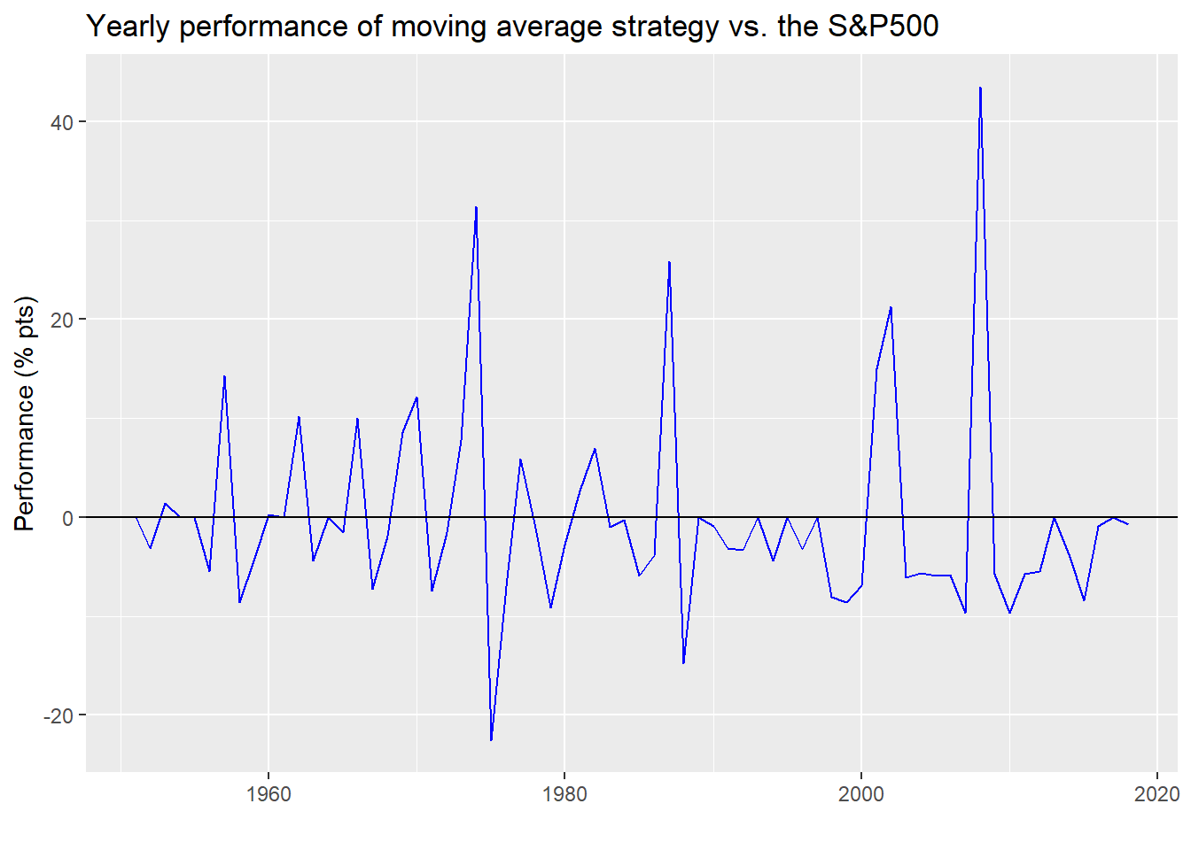
As one can see, the strategy underperforms the S&P500 more often than not. In fact, the strategy only outperforms the S&P 24% of the time as shown in the table below.
| Outperformance | Occurences (%) |
|---|---|
| Yes | 24 |
| No | 76 |
When you eyeball the graph it’s apparent that when the strategy outperforms it does so sizeably, while when it in underperforms it is of a much smaller magnitude. Said differently, it’s average outperformance is much greater than it’s average underperformance in absolute value, as shown in the table below. It’s like the trader’s old saw, “Keep your losses small and let your profits run.”
| Outperformance | Mean return (%) |
|---|---|
| Yes | 13.6 |
| No | -4.4 |
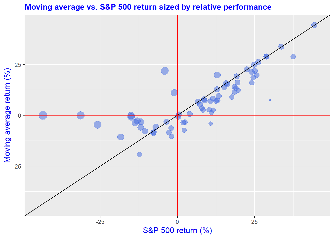
A different way to visualize relative performance of the strategy is to plot the moving average returns against the S&P 500, which we do below. We also include a 45o line that allows one to identify periods of outperformance based on position relative to the line (i.e., when the points are above the line, the strategy outperforms) and size of that outperformance (i.e., the larger the dot, the larger the outperformance). Evidently, the greatest outperformance tends to be when the S&P’s returns are siginifcantly negative, even though the strategy’s performance is close to zero. In other words, the strategy outperforms because it is out of the market!
There’s a bunch more ways we can cut the data to understand the sources of performance. But what we want to figure out is whether we’re more likely to meet our long-term return objective employing the moving average strategy over owning the the S&P 500.
To do that we’ll simulate performance based on predetermined parameters. Why do we do this insstead of simply using the past history? Mainly because the past is only one outcome that was heavily path dependent. Events could have turned out differently. We want to estimatte the likelihood what our the range of outcomes could be in the future.
Part of calculating that estimate requires us to choose the right parameters for our simulations. Those parameters are the average annual return and annual standard deviation, or volatiilty. But there is some discrection as to which average we can use. Should we use an average of the calendar years? Or maybe a rolling average of 12 months? Rolling 365 days? And should we use the total period or only part of it?
While it might not seem immediately obvious why these questions are important, once you see the results, it will be.
Let’s begin with using the calendar year averages, as shown in the table below, which we’ll use as our or risk and return parameters in the simulation.
| Strategy | Return (%) | Volatility (%) |
|---|---|---|
| Moving average | 7.3 | 12.6 |
| S&P 500 | 7.5 | 16.7 |
Using these averages, we calculate 100,000 cumulative returns and graph a density plot of the results.
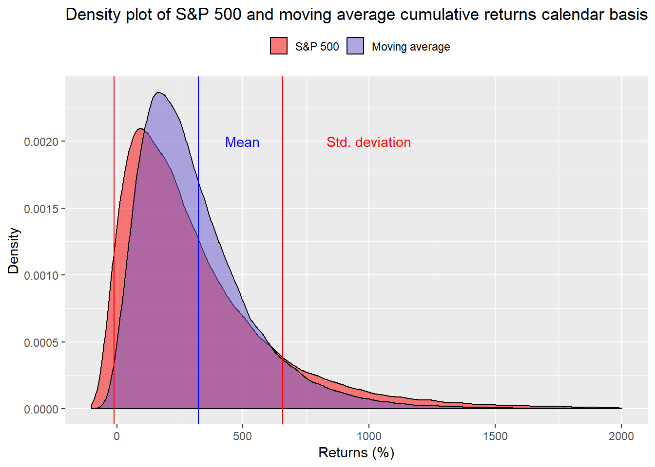
We won’t spend a lot of time deciphering the graph other than to point out the moving average strategy has fewer extreme results (fat tails) and does tend to cluster in a tighter range. We’ve removed some extremely high returns to make the graph more readable.
What is the probability the strategy falls short of its required 230% cumulative return we established in our previous post? About 43% That compares with the S&P 500 falling below the required return at 50%. A coint toss! Load the boat on the moving average stragegy!
Not so fast. Let’s look at a few more data points than over 65 years of calendar returns. While one wouldn’t expect market timing to matter all that much over a twenty year timeframe for a buy and hold strategy, it can if you are employing some sort of tactical allocation. Additionally, it’s unrealistic to expect every investor to buy on the first of the year. Capital flows into accounts at different times; folks deploy capital at different times too.
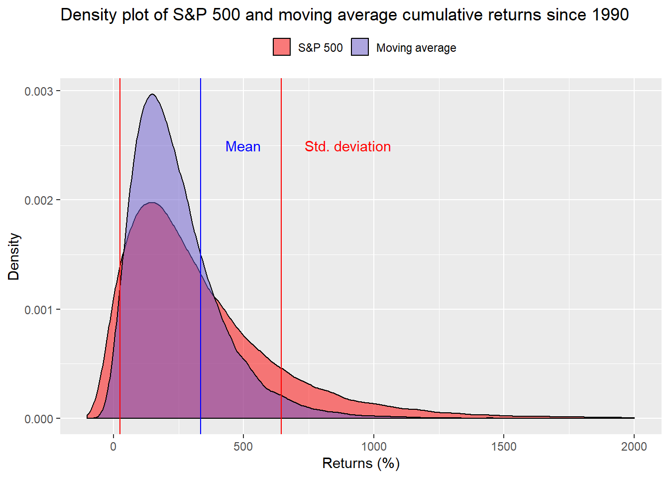
We now look the cumulative returns based on a rolling 12 month average of returns. First, we show the averages. Notice that average returns increase and volatility decreases slightly vs. our initial parameters. Is this enough to make a difference?
| Strategy | Return (%) | Volatility (%) |
|---|---|---|
| Moving average | 7.4 | 11.4 |
| S&P 500 | 7.6 | 16.1 |
When we run the simulations, it’s hard to see much difference vs. the prior graph.
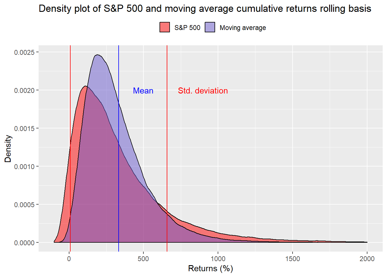
Nevertheless, the likelihood that one will fail to achieve the required returns falls 3 percentage points to 40% using the rolling averages of the moving average strategy. For the S&P, the probability of missing the target eases to 47% from 50% previously. Of course, the average returns and volatilities might be overstated since there’s a surfeit of repeated data. We’re aggregating a more realistic range of investment implementations at the expense of potentially overstating results. Still, the change in probabilities is not meaningful.1
What do we have thus far? We note that the probability we’ll fail to hit our required return target is lower with the moving average strategy than it is from simply the S&P 500. But also, recall that the moving average strategy did not outperform the S&P as much after 1990. What if we used only the returns generated after 1990 to simulate potential results? We may not be as likely to hit our target since the average annual return to the moving average strategy falls short of the S&P 500; although the volatility remmains lower, shown below.
| Strategy | Return (%) | Volatility (%) |
|---|---|---|
| Moving average | 6.4 | 11.3 |
| S&P 500 | 7.6 | 16.4 |
We run the simulations and show the density plot below. Note that in this series, the moving average is significantly more peaked than the S&P.
Based on averages since 1990, the moving average strategy misses the target 55% of the time! While the S&P only misses it 45% of the time. That leaves us in quandary. Which simulation is more likely to occur? Should we expect the future to be more like the last 68 years or more like only the last 30? Is the poor performance of strategy after 1990 an indicator that it no longer works or that it is out of favor as can happen to any strategy? How do we even answer these questions in a modestly rigorous fashion? That will have to wait until our next post. It’s okay to breath until then.
Here’s the code behind everything.
# Load package
library(tidyquant)

## Get the data
sp500 <- getSymbols("^GSPC", from = "1950-01-01", auto.assign = FALSE)
sp500 <- Cl(sp500)
sp_ret <- ROC(sp500)
sp_ret[is.na(sp_ret)] <- 0

# Create indicator and plot
sma <- SMA(sp500, n = 200)

# create signal
sig <- Lag(ifelse(sma$SMA < sp500, 1, 0))

# Calculate daily returns
ret <- ROC(sp500)*sig

# Create benchmark returns
sp_ret <- ROC(sp500)

# Name strategies
names(ret) <- "ret"
names(sp_ret) <- "sp_ret"

# Create tidy data frame
strat <- data.frame(date = index(ret),
                    ret = coredata(ret),
                    sp_ret = coredata(sp_ret)) %>%
  gather(key, value, - date) %>%
  filter(date > "1950-12-31")

# Create index of years
index <- data.frame(start_date = seq(as.Date("1951-01-01"), length = 49, by = "years"),
                    end_date = seq(as.Date("1970-12-31"), length = 49, by = "years"))

# Function to calculate 20-year cumulative return
perf_func <- function(df, start_date, end_date){
  data <- df %>%
    filter(date >= start_date, date <= end_date) %>%
    group_by(key) %>%
    summarise(perf = Return.cumulative(value)) %>%
    select(perf) %>%
    t()
  return(as.numeric(data))
}

# Create data frame and run For loop
perf <- data.frame(ret = rep(0,49), sp_ret = rep(0,49))
for(i in 1:49){
  perf[i,] <- perf_func(strat, index[i,1], index[i,2])
}


# Add years
perf <- perf %>%
  mutate(year = year(index$end_date))

# Outperformance
tot_opf <- perf %>%
  summarise(prop = round(mean(ret > sp_ret),2)*100) %>%
  as.numeric()

part_opf <- perf %>%
  filter(year >= "1990") %>%
  summarise(prop = round(mean(ret > sp_ret),2)*100) %>%
  as.numeric()

# Table by year
ret_year <- strat %>%
  mutate(year = year(date)) %>%
  group_by(key, year) %>%
  filter(year < "2019") %>%
  summarize(value = Return.cumulative(value)*100) %>%
  spread(key, value) %>%
  data.frame()

# Graph year performance
ret_year %>%
  mutate(perf = ret-sp_ret) %>%
  ggplot(aes(year, perf)) +
  geom_line(color = "blue") +
  geom_hline(yintercept = 0, color = "black") +
  labs(y = "Performance (%)",
       x = "",
       title = "Yearly performance of moving average strategy vs. the S&P500")

times_out <- round(sum(ifelse(ret_year$ret >ret_year$ sp_ret, 1, 0))/nrow(ret_year),2)*100

# Count out performance
ret_year %>%
  mutate(Outperformance = ifelse(ret > sp_ret, "Yes", "No")) %>%
  group_by(Outperformance) %>%
  summarise(`Occurences (%)` = round(n()/nrow(ret_year),2)*100) %>%
  arrange(`Occurences (%)`) %>%
  knitr::kable()

# AVerage performance
ret_year %>%
  mutate(Outperformance = ifelse(ret > sp_ret, "Yes", "No")) %>%
  group_by(Outperformance) %>%
  mutate(perf = ret - sp_ret) %>%
  summarise(`Mean return (%)` = round(mean(perf),1)) %>%
  arrange(desc(`Mean return (%)`)) %>%
  knitr::kable()

# Graph of Strategy performance vs. S&P ret, sized by relative performance of strategy

ret_year %>%
  mutate(perf = ret-sp_ret) %>%
  ggplot(aes(sp_ret, ret, size = perf)) +
  geom_point(color = "royalblue", alpha = 0.5) +
  geom_abline(slope = 1, intercept = 0, color = "black") +
  geom_vline(xintercept = 0, color = "red") +
  geom_hline(yintercept = 0, color = "red") +
  xlim(c(-45,45)) + ylim(c(-45, 45)) +
  labs(y = "Moving average return (%)",
       x = "S&P 500 return (%)",
       title = "Moving average vs. S&P 500 return sized by relative performance") +
  theme(legend.position = "none", plot.title = element_text(size = 12,
                                                            color = "blue",
                                                            face = "bold"),
        axis.title = element_text(size = 12, color = "blue2"))

# Calendar averages
strat %>%
  mutate(year = year(date)) %>%
  mutate(key = case_when(key == "ret" ~ "Moving average",
                         key == "sp_ret" ~ "S&P 500")) %>%
  rename("Strategy" = key) %>%
  group_by(Strategy, year) %>%
  filter(year < "2019") %>%
  summarize(value = Return.cumulative(value)*100) %>%
  summarize("Return (%)" = round(mean(value),1),
            "Volatility (%)" = round(sd(value),1)) %>%
  knitr::kable()


# simulate function for returns
return_func <- function(years, return, risk){
  asset <- rnorm(years, return, risk)
  cum_ret <- Return.cumulative(asset)
  return(cum_ret)
}

# Replicate
set.seed(123)
strat_mu <-mean(ret_year$ret)/100
strat_sigma <- sd(ret_year$ret)/100

sp_mu <- mean(ret_year$sp_ret)/100
sp_sigma <- sd(ret_year$sp_ret)/100

strat_out <- replicate(100000, return_func(20, strat_mu, strat_sigma))
sp_out <- replicate(100000, return_func(20, sp_mu, sp_sigma))
comp <- data.frame(strat_out, sp_out)
comp_mu <- mean(comp$sp_out)
comp_sigma <- sd(comp$sp_out)

# Graph overlapping density plot
comp %>%
  gather(key, value) %>%
  ggplot(aes(value*100, fill = key)) +
  geom_density(alpha = 0.5) +
  geom_vline(xintercept = comp_mu*100, color = "red")+
  geom_vline(xintercept = (comp_mu + comp_sigma)*100, color = "blue") +
  geom_vline(xintercept = (comp_mu - comp_sigma)*100, color = "blue") +
  xlim(c(-100, 2000)) +
  labs(x = "Returns (%)",
       y = "Density",
       title = "Density plot of S&P 500 and moving average cumulative returns calendar basis") +
  scale_fill_manual("", labels = c("S&P 500", "Moving average"),
                     values = c("red", "slateblue")) +
  theme(legend.position = "top")

# How likely are we to fall short of our target
strat_below <- round(mean(comp$strat_out < 2.3),2)*100
sp_below <- round(mean(comp$sp_out < 2.3),2)*100

# How often below zero?
strat_zero <- round(mean(comp$strat_out < 0),2)*100
sp_zero <- round(mean(comp$sp_out < 0),2)*100

# Create index
year_idx <- data.frame(start_date = seq(as.Date("1951-01-01"),
                                        length = 805,
                                        by = "months"),
                       end_date = seq(as.Date("1952-01-01"),
                                      length = 805,
                                      by = "months"))

# Calculate returns
year_perf <- data.frame(ret = rep(0,805), sp_ret = rep(0,805))
for(i in 1:805){
  year_perf[i,] <- perf_func(strat, year_idx[i,1], year_idx[i,2])
}

# Add years to year_perf
year_perf <- year_perf %>%
  mutate(year = year_idx$end_date) %>%
  select(year, ret, sp_ret)

# Average table
year_perf %>%
  gather(key = "Strategy", value, - year) %>%
    mutate(Strategy = case_when(Strategy == "ret" ~ "Moving average",
                         Strategy == "sp_ret" ~ "S&P 500")) %>%
  group_by(Strategy) %>%
  summarize("Return (%)" = round(mean(value),3)*100,
            "Volatility (%)" = round(sd(value),3)*100) %>%
  knitr::kable()

# Simulate with larger data set
strat_mu_yr <- mean(year_perf$ret)
strat_sigma_yr <- sd(year_perf$ret)

sp_mu_yr <- mean(year_perf$sp_ret)
sp_sigma_yr <- sd(year_perf$sp_ret)

set.seed(123)
strat_out_yr <- replicate(100000, return_func(20, strat_mu_yr, strat_sigma_yr))
sp_out_yr <- replicate(100000, return_func(20, sp_mu_yr, sp_sigma_yr))

comp_yr <- data.frame(strat_out_yr, sp_out_yr)
comp_yr_mu <- mean(comp_yr$sp_out_yr)
comp_yr_sigma <- sd(comp_yr$sp_out_yr)

# Graph overlapping density plot
comp_yr %>%
  gather(key, value) %>%
  ggplot(aes(value*100, fill = key)) +
  geom_density(alpha = 0.5) +
  geom_vline(xintercept = comp_yr_mu*100, color = "red")+
  geom_vline(xintercept = (comp_yr_mu + comp_yr_sigma)*100, color = "blue") +
  geom_vline(xintercept = (comp_yr_mu - comp_yr_sigma)*100, color = "blue") +
  xlim(c(-100, 2000)) +
  labs(x = "Returns (%)",
       y = "Density",
       title = "Density plot of S&P 500 and moving average cumulative returns") +
  scale_fill_manual("", labels = c("S&P 500", "Moving average"),
                    values = c("red", "slateblue")) +
  theme(legend.position = "top")

# How likely are we to fall short of our target
strat_below_yr <- round(mean(comp_yr$strat_out_yr < 2.3),2)*100
sp_below_yr <- round(mean(comp_yr$sp_out_yr < 2.3),2)*100

# How often below zero?
strat_zero_yr <- round(mean(comp_yr$strat_out_yr < 0),2)*100
sp_zero_yr <- round(mean(comp_yr$sp_out_yr < 0),2)*100

# Average table
year_perf %>%
  gather(key = "Strategy", value, - year) %>%
  filter(year >= "1990-01-01") %>%
  mutate(Strategy = case_when(Strategy == "ret" ~ "Moving average",
                         Strategy == "sp_ret" ~ "S&P 500")) %>%
  group_by(Strategy) %>%
  summarize("Return (%)" = round(mean(value),3)*100,
            "Volatility (%)" = round(sd(value),3)*100) %>%
  knitr::kable()

# since 1990
strat_mu_90 <- mean(year_perf[year_perf$year >= "1990-01-01",2])
strat_sigma_90 <- sd(year_perf[year_perf$year >= "1990-01-01",2])

sp_mu_90 <- mean(year_perf[year_perf$year >= "1990-01-01",3])
sp_sigma_90 <- head(year_perf[year_perf$year >= "1990-01-01",3])

strat_out_90 <- replicate(100000, return_func(20, strat_mu_90, strat_sigma_90))
sp_out_90 <- replicate(100000, return_func(20, sp_mu_90, sp_sigma_90))

comp_90 <- data.frame(strat_out_90, sp_out_90)
comp_90_mu <- mean(comp_90$sp_out_90)
comp_90_sigma <- sd(comp_90$sp_out_90)

# Graph overlapping density plot
comp_90 %>%
  gather(key, value) %>%
  ggplot(aes(value*100, fill = key)) +
  geom_density(alpha = 0.5) +
  geom_vline(xintercept = comp_90_mu*100, color = "red")+
  geom_vline(xintercept = (comp_90_mu + comp_90_sigma)*100, color = "blue") +
  geom_vline(xintercept = (comp_90_mu - comp_90_sigma)*100, color = "blue") +
  xlim(c(-100, 2000)) +
  labs(x = "Returns (%)",
       y = "Density",
       title = "Density plot of S&P 500 and moving average cumulative returns") +
  scale_fill_manual("", labels = c("S&P 500", "Moving average"),
                    values = c("red", "slateblue")) +
  theme(legend.position = "top")

# How likely are we to fall short of our target
strat_below_90 <- round(mean(comp_90$strat_out_90 < 2.3),2)*100
sp_below_90 <- round(mean(comp_90$sp_out_90 < 2.3),2)*100

# How often below zero?
strat_zero_90 <- round(mean(comp_90$strat_out_90 < 0),2)*100
sp_zero_90 <- round(mean(comp_90$sp_out_90 < 0),2)*100
Apologies to the mathematicians reading this. The data are likely to be auto-correlated and feature a whole host of other issues that would make using a simple average a less robust estimator. But trying to explain all that is beyond the scope (and space!) of this article.↩