Playing with averages
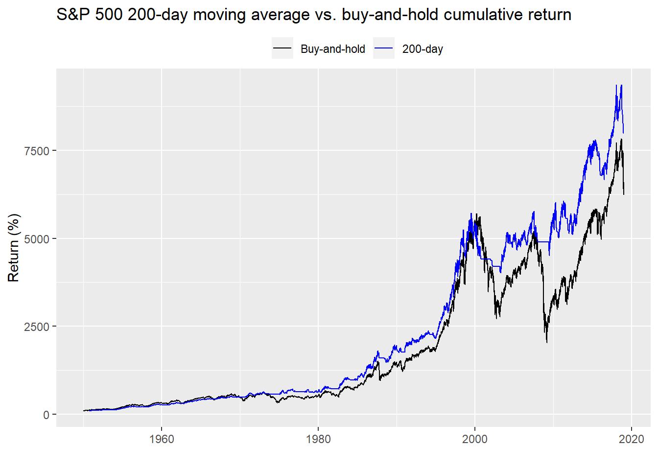
In a previous post we compared the results from employing a 200-day moving average tactical allocation strategy to a simple buy-and-hold investment in the S&P500. Over the total period, the 200-day produced a higher cumulative return as well as better risk-adjusted returns. However, those metrics did erode over time until performance was essentially in line or worse since 1990.
While there’s still some more work to do on understanding the drivers of performance for the 200-day strategy. We’re going to shift our focus a bit to examine alternate (but still relatively stratightforward) tactical allocations. This is where the power of data science will come in handy to allow us to analyze a whole series of allocations in relatively short order.
In this post, we’ll check to see if there might be a better signal than the 200-day moving average. We’ll look at mean, cumulative, and risk-adjusted returns. But to refresh our memories let’s first look at the long run cumulative return chart for the 200-day moving average and buy-and-hold allocation for the S&P 500.
And just for the heck of it, let’s look at the average annual returns by decade.
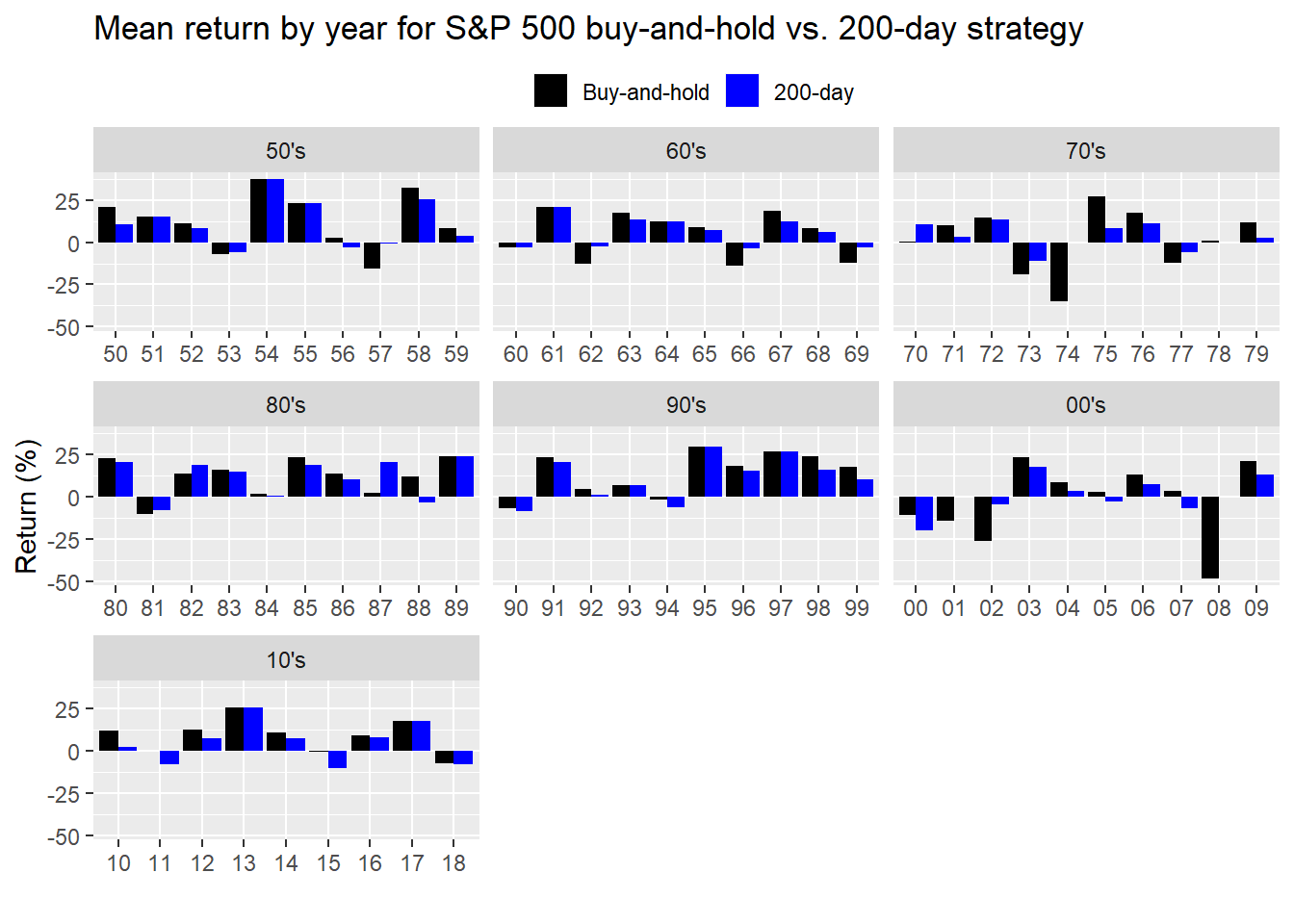
Clearly, a bit of an eye-test, but we can see that most of the time, the buy-and-hold outperforms the 200-day on the upside, while the 200-day outperforms the buy-and-hold on the down. Why is this the case? Since the 200-day represents attempts to capture the underyling trend by smoothing the data over a long period of time, buy and sell signals will be generated infrequently. Indeed, there will often be a significant lag between when the 200-day produces a signal relative to how much the market will have moved simply because the weight of the past 200 days of data will be slow to react to recent changes. To counteract that lag, one can use a shorter time frame or give more weight to nearer data. In both cases, the trade-off for a faster reaction may confuse noise with signal. In other words, choppiness in the data will produce many false signals that will be bad for your wallet!
Nonetheless, there’s nothing magical about the 200-day moving average other than convention and a couple of studies from well-respected professors. Could a different period moving average produce better results? Let’s test that.
Behind the scenes we’ll create a function that allows us to test various moving average signals and then loop through different moving average windows. We’ll also include the 200-day and buy-and-hold for reference. We’ll first look at average annualized returns.
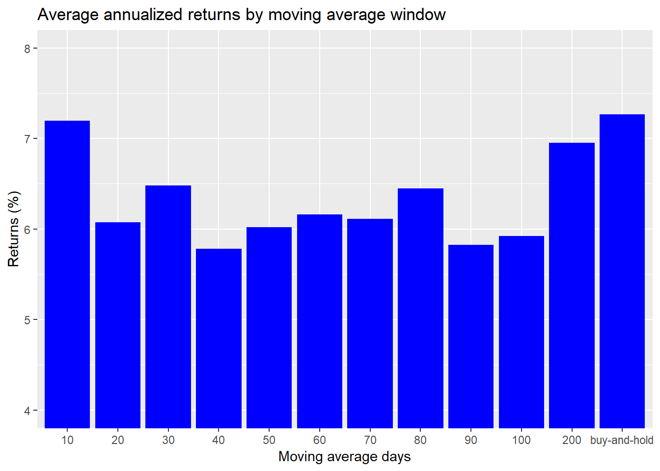
Interesting, over the entire period, only the 10-day moving average tactic approximated the buy-and-hold. The 200-day was actually slightly worse than buy-and-hold. What about risk-adjusted returns?
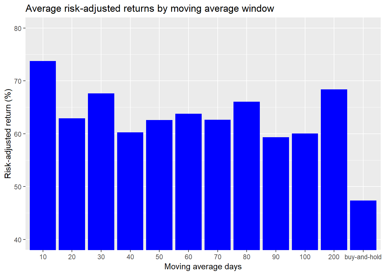
Every tactic produced better risk-adjusted returns than buy-and-hold. But the 10-day moving average was the clear winner. This begs the question as to whether the reults were persistent across time. Let’s run through the decades to see how the various tactics would fare.
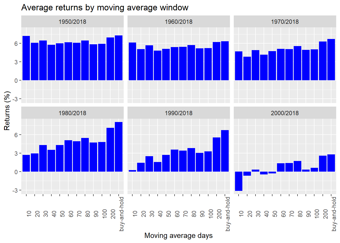
Wow that’s interesting. Over time the average annual return of the tactical allocations has declined meaningifully, especially relative to buy-and-hold. What about risk-adjusted returns?
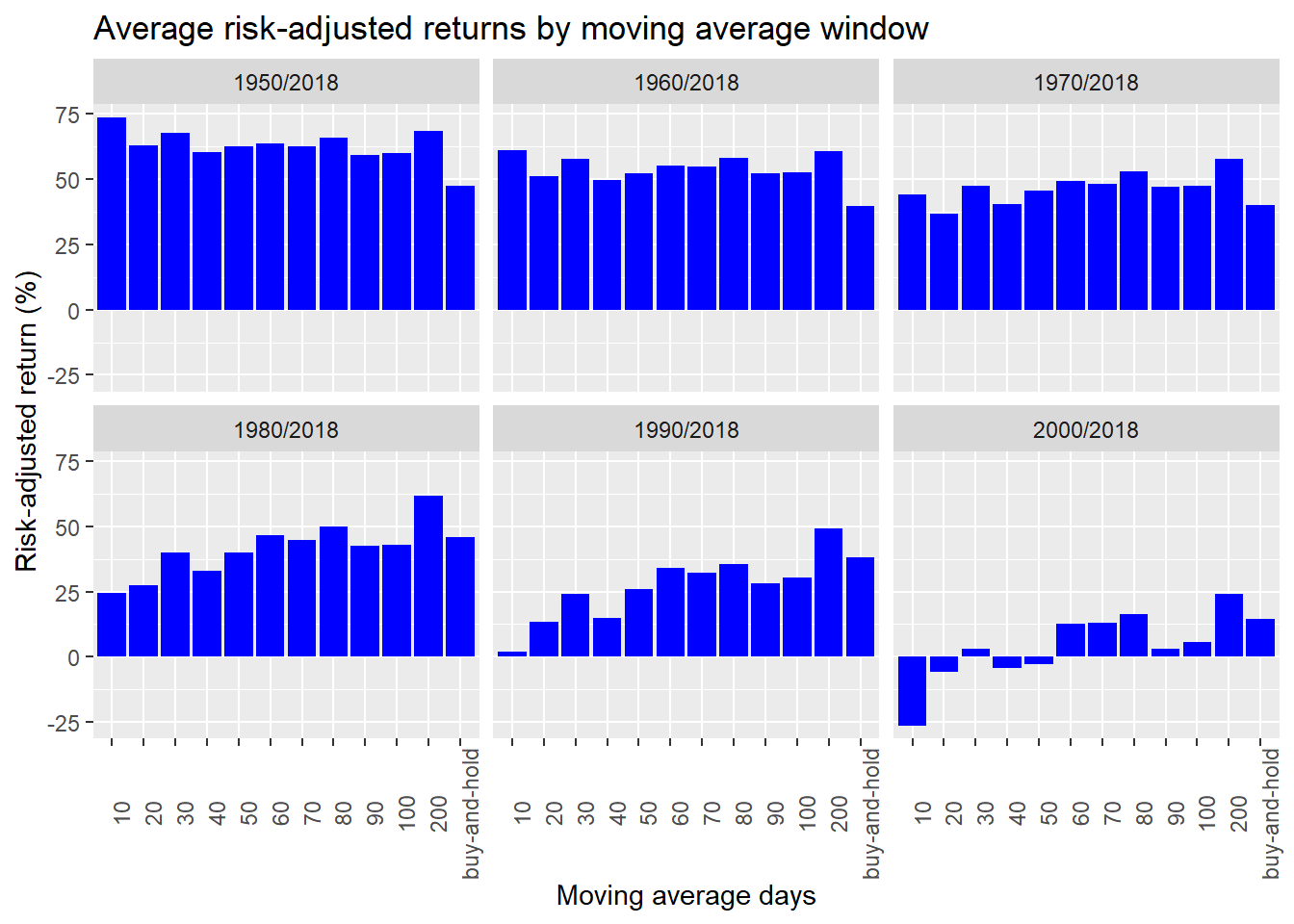
Another intersting group of results. Risk-adjusted returns erode over time and erode relative to buy-and-hold. Let’s drill down a bit to see which produced the best overall return by period.
| Period | Tactic | Return (%) |
|---|---|---|
| 1950/2018 | buy-and-hold | 7.3 |
| 1960/2018 | buy-and-hold | 6.3 |
| 1970/2018 | buy-and-hold | 6.7 |
| 1980/2018 | buy-and-hold | 8.0 |
| 1990/2018 | buy-and-hold | 6.7 |
| 2000/2018 | buy-and-hold | 2.8 |
The buy-and-hold allocation produced the highest average annualized return over each period. And what about risk-adjusted returns?
| Period | Tactic | Risk-adjusted return (%) |
|---|---|---|
| 1950/2018 | 10-day | 73.8 |
| 1960/2018 | 10-day | 61.2 |
| 1970/2018 | 200-day | 58.0 |
| 1980/2018 | 200-day | 61.9 |
| 1990/2018 | 200-day | 49.2 |
| 2000/2018 | 200-day | 24.1 |
This time it appears the 200-day generally produced better risk-adjusted returns on four out of the six periods. On this initial reading, it appears the 200-day’s risk-adjusted outperformance tends to persist over time. But these are only preliminary results. We need to employ some more sophisticated tests to verify that both the outperformance and persistence of outperformance are significant. That will require another post. Until then, here is the code behind the results.
# Load package
library(tidyquant)

# Get the data
sp <- getSymbols("^GSPC", from = "1950-01-01", to = "2018-12-31", auto.assign = FALSE)
sp <- Ad(sp) %>% `colnames<-`("sp")

# Moving average function
mov_avg_func <- function(df, window, increment){
  # Create moving average
  sma <- SMA(df, n = window)

  # Create up and down increments
  up_inc <- 1 + increment
  down_inc <- 1 - increment

  # Create index vectors for signal
  open <- sma$SMA != 0 & sma$SMA < df & df/sma$SMA > up_inc
  close <- sma$SMA > df & df/sma$SMA < down_inc
  hold_open <- sma$SMA > df & df/sma$SMA > down_inc
  hold_close <- sma$SMA < df & df/sma$SMA < up_inc

  # Create signal. Order of indices is important!
  signal <- as.xts(rep(NA, nrow(sma)), order.by = index(sma))
  signal[open] <- 1
  signal[close] <- 0
  signal[hold_open] <- 1
  signal[hold_close] <- 0

  # Lag signal for proper return calc. Note: Quantmod Lag sometimes acts stranged
  signal <- Lag(signal)

  # Create return object with bench mark
  strat <- ROC(df)*signal
  names(strat) <- "strat"

  bench <- ROC(df)
  names(bench) <- "bench"

  # Merge and return
  results <- merge(strat, bench)
  results
}

# Run 200 day
ma_200 <- mov_avg_func(sp, 200, 0)
ma_200_df <- data.frame(date = index(ma_200), coredata(ma_200))

# Graph 200 day
ma_200_df %>%
  gather(key,value, -date) %>%
  filter(!is.na(value)) %>%
  group_by(key) %>%
  mutate(value = cumprod(value+1)) %>%
  ggplot(aes(date, value*100, color = key)) +
  geom_line() +
  labs(y = "Return (%)",
       x = "",
       title = "S&P 500 200-day moving average vs. buy-and-hold cumulative return") +
  scale_color_manual("", labels = c("Buy-and-hold", "200-day"),
                     values = c("black", "blue")) +
  theme(legend.position = "top", legend.box.spacing = unit(0.05, "cm"))

# Create facet labels
years <- seq(1950, 2010, 10)
facet_labels <- c(paste(substring(years,3), "s", sep ="'"))
names(facet_labels) <- years

# Graph averaage annual returns by decade
ma_200_df %>%
  gather(key, value, -date) %>%
  mutate(year = year(date),
         decade = trunc(year/10,0)*10) %>%
  group_by(key, year, decade) %>%
  summarise(value = mean(value, na.rm = TRUE)*25200) %>%
  ggplot(aes(substring(year,3), value, fill = key)) +
  geom_bar(position = "dodge", stat = "identity") +
  facet_wrap(~ decade,
             scales = "free_x",
             labeller = as_labeller(facet_labels)) +
  scale_fill_manual("",
                    labels = c("Buy-and-hold", "200-day"),
                    values = c("black", "blue")) +
  theme(legend.position = "top",
        legend.box.spacing = unit(0.05, "cm"),
        legend.key.size = unit(0.5, "cm")) +
  labs(title = "Mean return by year for S&P 500 buy-and-hold vs. 200-day strategy",
       x = "",
       y = "Return (%)")

## Run moving average strategy on different averages

# Create list and iterate function
mov_avg_test <- list()
for(i in 1:12){
  if(i < 11){
    mov_avg_test[[i]] <- mov_avg_func(sp, i*10, 0)$strat
  }else if(i == 11){
    mov_avg_test[[i]] <- mov_avg_func(sp, 200, 0)$strat
  }else{
    mov_avg_test[[i]] <- mov_avg_func(sp, i*10, 0)$bench
  }
}

mov_avg_names <- c(paste(seq(10,100,10),"d", sep = ""), "200d", "buy-and-hold")
names(mov_avg_test) <- mov_avg_names

# Create reward-to-risk function
reward_risk <- function(df, period){
  avg <- mean(df, na.rm = TRUE)
  stdev <- sd(df, na.rm = TRUE)
  reward_risk <- avg/stdev*sqrt(period)
  reward_risk
}

# Create data frame for results analysis
returns <- data.frame(window = factor(c(c(1:10)*10, 200, "buy-and-hold"),
                                      levels = c(c(1:10)*10, 200, "buy-and-hold")),
                      mean_returns = rep(0,12),
                      cum_returns = rep(0,12),
                      rew_risk = rep(0,12))

for(i in 1:12){
  returns[i,2] <- mean(mov_avg_test[[i]], na.rm = TRUE)*252
  returns[i,3] <- prod(mov_avg_test[[i]]+1, na.rm = TRUE)
  returns[i,4] <- reward_risk(mov_avg_test[[i]], period = 252)
}

# Graph returns
returns %>%
  ggplot(aes(window, mean_returns*100)) +
  geom_bar(stat = "identity", fill = "blue") +
  labs(title = "Average annualized returns by moving average window",
       y = "Returns (%)",
       x = "Moving average days") +
  coord_cartesian(ylim = c(4,8))

# Graph risk-adjusted returns
returns %>%
  ggplot(aes(window, rew_risk*100)) +
  geom_bar(stat = "identity", fill = "blue") +
  labs(title = "Average risk-adjusted returns by moving average window",
       y = "Risk-adjusted return (%)",
       x = "Moving average days") +
  coord_cartesian(ylim = c(40,80))

## Examine moving average strategies over different periods

# Create list of data frames for multiple periods

# Create periods of interest
periods <- c()
decade <- seq(1950,2000, 10)

for(i in 1:6){
  periods[i] <- paste(decade[i], "2018", sep = "/")
}

# Create data frames within list for periods of interest
returns_decade <- list()
for(i in 1:6){
  returns_decade[[i]] <- data.frame(window = factor(c(c(1:10)*10, 200, "buy-and-hold"),
                                                    levels = c(c(1:10)*10, 200, "buy-and-hold")),
                                    mean_returns = rep(0,12),
                                    cum_returns = rep(0,12),
                                    rew_risk = rep(0,12))
  for(j in 1:12){
    returns_decade[[i]][j,2] <- mean(mov_avg_test[[j]][periods[i]], na.rm = TRUE)*252
    returns_decade[[i]][j,3] <- prod(mov_avg_test[[j]][periods[i]]+1, na.rm = TRUE)
    returns_decade[[i]][j,4] <- reward_risk(mov_avg_test[[j]][periods[i]], period = 252)
  }
}

names(returns_decade) <- periods

# Merge list of data frames into one data frame
returns_decade_df <- returns_decade %>%
  bind_rows(.id = "periods")


# Graph returns
returns_decade_df %>%
  ggplot(aes(window, mean_returns*100)) +
  geom_bar(stat = "identity", fill = "blue") +
  facet_wrap(~ periods) +
  labs(title = "Average returns by moving average window",
       y = "Returns (%)",
       x = "Moving average days") +
  theme(axis.text.x = element_text(angle = 90))

# Graph risk-adjusted returns
returns_decade_df %>%
  ggplot(aes(window, rew_risk*100)) +
  geom_bar(stat = "identity", fill = "blue") +
  facet_wrap(~ periods) +
  labs(title = "Average risk-adjusted returns by moving average window",
       y = "Risk-adjusted return (%)",
       x = "Moving average days") +
  theme(axis.text.x = element_text(angle = 90))

# Max returns by decade
returns_decade_df %>%
  group_by(periods) %>%
  filter(mean_returns == max(mean_returns)) %>%
  select(periods, window, mean_returns) %>%
  mutate(mean_returns = round(mean_returns,3)*100) %>%
  rename("Period" = periods,
         "Tactic" = window,
         "Return (%)" = mean_returns) %>%
  knitr::kable(caption = "Highest average annualized return by period")

# Max risk-adjusted returns by decade
returns_decade_df %>%
  group_by(periods) %>%
  filter(rew_risk == max(rew_risk)) %>%
  select(periods, window, rew_risk) %>%
  mutate(rew_risk = round(rew_risk,3)*100,
         window = paste(window, "day", sep = "-")) %>%
  rename("Period" = periods,
         "Tactic" = window,
         "Risk-adjusted return (%)" = rew_risk) %>%
  knitr::kable(caption = "Best risk-adjusted return by period")