Detour: correlation
In our last post, we asked the simple question of whether an investor is better off being diversified if he or she doesn’t know in advance how a stock is likely to perform. We showed some graphs that suggested diversification lowered risk (or, more precisely, volatility), but this came at the expense of accepting less than maximal returns. We then showed that a diversified portfolio was able to produce better risk-adjusted returns on 8 out of 10 of the stocks we had randomly generated. But we reasoned that, while these results were encouraging, they didn’t answer the question conclusively because we only used one portfolio. We aruged that we would need to create a large sample of portfolios to see if by analyzing the risk/return proflles of those samples we’d reach a more robust answer.
However, before we do this we want to explain why diversification worked in our simple portfolio example. For that we need to take a detour into correlation.
Correlation and beyond
As a concept, correlation is relatively straightforward. For stocks, if two stocks tend to move in the same diretion they’re correlated; and if they don’t, they’re not. How closely they move together (in terms of frequency and amplitude) determines the magnitude of that correlation. Mathematically, correlation runs from -1 (perfectly negatively correlated) to 1 (perfectly positively correlate). This scale makes it relatively easy to conceptualize even without understanding the math behind it. What correlation means for a portfolio is that if the stocks in the portfolio are not perfectly positively correlated, then the overall risk of the portfolio is lower than any one stock. Why is that? While some stocks are zigging, others are zagging or zigging even less. Hence, if you’ve got some stocks going down, others are going up to offset it.
Seems simple enough, but there are nuances. First, correlation has its drawbaks. It’s nice when a bunch of your stocks are going down, there are some that aren’t. It’s not so nice when you have a few stocks soaring, but the rest are plummetting, offsetting those juicy gains. Thus, while it is good to have some stocks that aren’t highly correlated with others, you don’t want a portfolio in which many of the stocks are negatively correlated; otherwise, your returns would be negligible, since every move up would be countered by an almost equal move down. In reality, it becomes increasingly unlikely that you could create such a portfolio once you move beyond two assets. Still performance drag is an issue. 1
This issue leads to a second nuance. That is, there isn’t an ideal correlation for the assets in the portfolio. You don’t want them all perfectly correlated. But what is the right amount of correlation? Professionals construct portfolios to optimize returns for a given level of risk or vice-versa. Correlation is an input to this model, but it is not being optimized. Importantly, correlations change, which affects the risk of the portfolio. Imagine constructing a portfolio which has a nice balance of uncorrelated assets only to find those correlations have changed after a few months! Clearly, this is an important issue, but beyond the scope of the current article. 2
Another nunace is that one doesn’t need to have negatively correlated assets to benefit from diversification. Simply having assets that are less positively correlated lowers portfolio volatility. That doesn’t mean it lowers the probability of loss, a different definition of risk, but that too is a separate topic. Let’s return to our main focus: understanding how correlation supports diversification
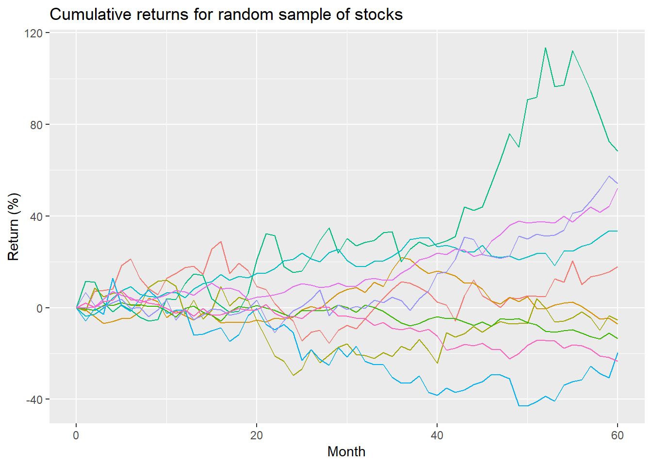
Recall the chart of our random group of stocks we created.
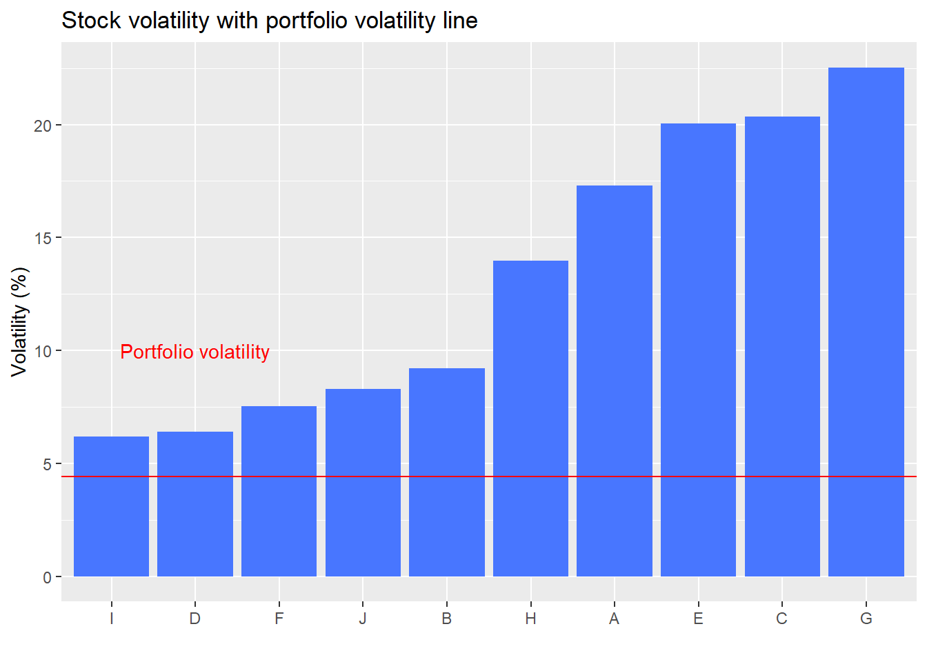
And here’s the volatility chart, which shows the portfolio volatility (the red line) as lower than the volatility of any individual stock.
So what drives diversification anyway?
If you wondered why our toy portfolio had lower volatility than any of the individual stocks it was because of correlation. While half the stocks were higher at the end of the period, the other half were lower, which means the correlations of many of the stocks with each other was negative. In addition, among the stocks that moved in the same direction, the amount they moved and the path they took was also sufficiently different to result in lower correlations (an example of the third nuance mentioned above).
Let’s build the intuition on how correlation helps diversification lower portfolio volatility over a range of correlations. We’ll start with a simple two stock portfolio, assuming both stocks have the same risk and return profiles and assuming an equal-weighting of those stocks. Then we’ll simulate the range of portfolio volatilities based on different correlation coefficients.
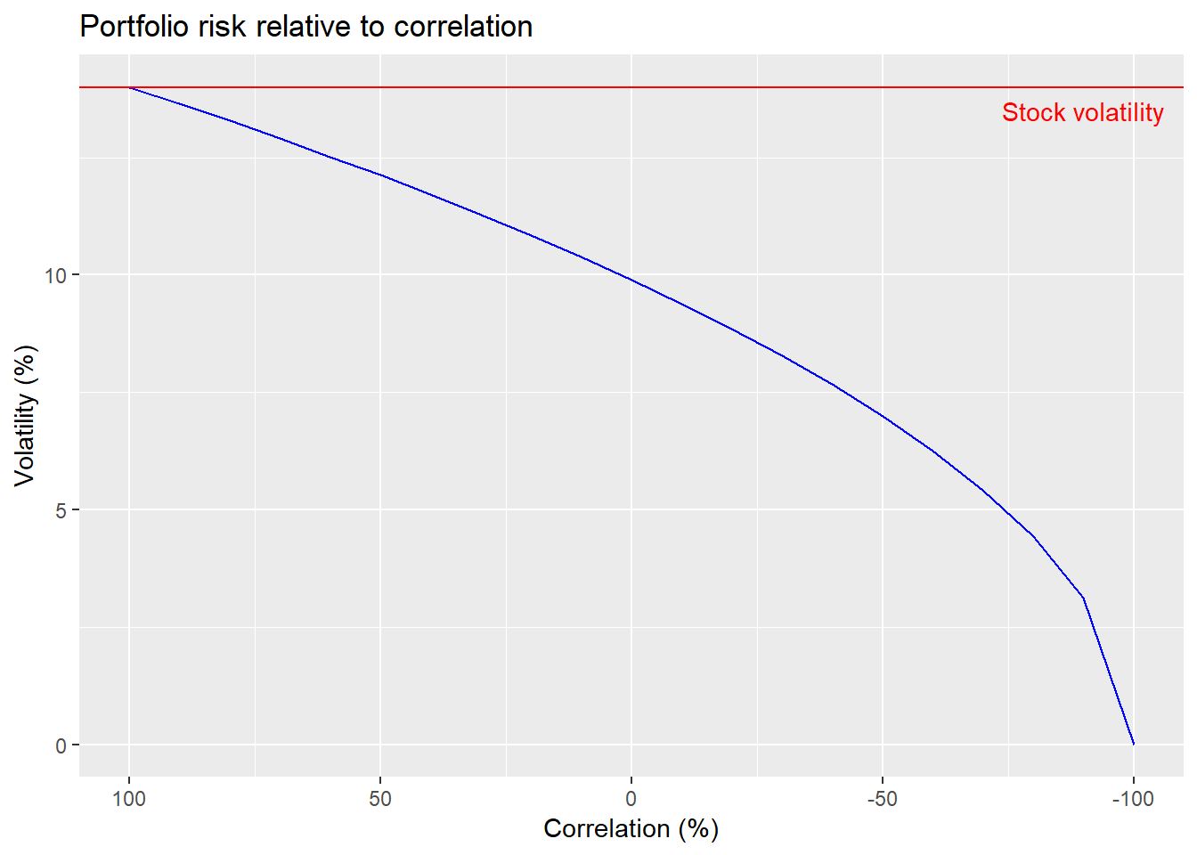
As the graph shows, when the two stocks are perfectly positively correlated, portfolio volatility equals stock volatility. When they’re perfectly negatively correlated, portfolio volatility is zero.3 It would, of course, be different than zero if the two stocks didn’t have exactly the same volatility and weren’t equal-weighted. We reversed the order of the x-axis to make the decline in volatility easier to read. Another important point is that the decline in volatility isn’t linear. It’s close to linear as correlation declines from 100% to zero, but then accelerates thereafter.
What happens if you add a third stock to the portfolio? The answer is it depends on the correlation of the initial stocks and how the third stock correlates with those stocks. It is difficlut to show this across a broad range of correlations without creating mathematically impossible scenarios. We’ll use three cases in which the stocks in the original portfolio have negative (-50%), zero, or positive correlation (50%). The stock we add will have a 50% correlation with the first stock in the two stock portfolio and a range of possible correlations with the second stock, as permitted by the math.4
The horizontal line represents the volatility of the two stock portfolio for its respective correlation. The sloping line is the portfolio volatility based on the correlation of the additonal stock to the second stock in the portfolio. Recall the correlation between the additional stock and the first stock in the portfolio is 50%.
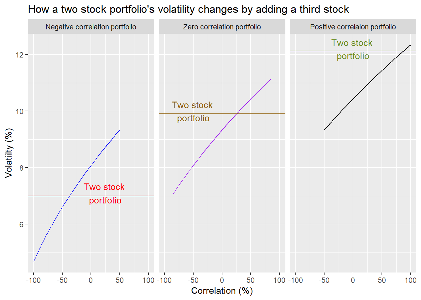
A few takeaways from these graphs. The more positively correlated the stocks, the higher the risk. Adding another stock often lowers volatility, but not in all cases. But that addition also can cause the volatitlies of the portfolios to overlap, suggesting a wider range of risk. Another takeaway is that if you have a negatively correlated portfolio, adding a stock with positive correlation to one of the stocks only results in lower portfolio volatility if it is sufficiently negatively correlated with the other stock, around -40% or less. On the other hand, if the portfolio correlation is zero or positive, even adding a stock with postive correlation can lower portfolio volatility.
Based on this we can make some provisional generalizations. First, if the assets in your portfolio already exhibit negative correlation, adding a postively correlated asset with one of the the other assets will likely increase portfolio volatility unless it is negatively correlated with the other assets in the portfolio to almost the same magnitude as its positive correlation.
The second generalization is if there is little correlation among the assets of the portfolio, then adding another asset that is positively correlated to one of the former assets can lower total portfolio volatility so as long as its correlation to the remaining assets isn’t overly large. In this case, the correlation can’t be greater than 17%.
Third generalization. If the assets in the initial portfolio already exhibit positive correlation, adding another asset positively correlated to portion of the existing assets generally lowers portfolio volatility so long as its correlation with the other assets is not excessive; not greater than 85% in this case.
An easy way to see this in terms of likelihood that portfolio volatility will decline is shown below.
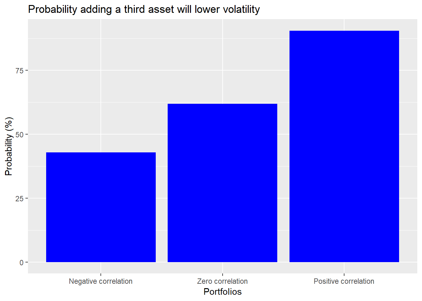
What’s the headline conclusion? When you combine stocks that aren’t perfectly positively correlated the overall volatility of your portfolio goes down. However, when you already own stocks that aren’t perfectly positively correlated and you add a new stock to that portfolio, how much volatility declines (if at all) depends on the magnitude and sign of the new stock’s correlation with the rest of the portfolio.
Why should you care about correlation? When constructing a portfolio you look at the expected risk and return of potential assets. The total risk of the portfolio is, of course, determined by the expected risk of each asset, modified by the correlation of each asset with every other asset, aggregated according to how much exposure you decide to have to each asset. For a three asset portfolio, there are three different correlations you need to know. For a four asset portfolio, there are six correlations, and for five asssets, 10 correlations. The amount of correlations you need to attend to increases significantly as you add more assets.
Understanding how a portfolio’s risk might change becomes relatively complex once you go beyond three assets. Why? Because the pairs of correlations increases. Recall the three stock portfolio. When we think of the interactions of those three stocks we only need to think about three pairs of correlations. That’s relatively easy to conceptualize like imagining which direction three balls might bounce if you dropped them from the second floor window of your house. Whichever direction they bounce in and what that direction is relative to the others is relatively easy to see your mind’s eye? Four balls it becomes more difficult. Four balls over multiple bounces? Maybe Rain Man could do it. Not sure about anyone else.
That returns us to our original question: is an investor better off being diversified if he or she doesn’t know in advance how a stock or group of stocks is likely to perform? The question implies not only not knowing how the stocks will perform, but also how correlated they’ll be with one another. This uncertainty surround correlation adds a further complication. Based on what we’ve shown in the previous post and what we’ve learned in this post about how correlation underpins diversification, our provisional vote in favor of diversification has weakened a bit. In some cases, adding a stock to a portfolio with the hope of lowering volatility coud have the opposite effect. How likely that is we’ll leave to another post where we’ll return to the original portfolio and run simulations with different correlation assumptions.
Until next time, here is the underlying code we used for this post.
# Load package
library(tidyquant)

# Create toy portfolio
set.seed(123)
mu <- seq(-.03/12,.08/12,.001)
sigma <- seq(0.02, 0.065, .005)

mat <- matrix(nrow = 60, ncol = 10)
for(i in 1:ncol(mat)){
  mu_samp <- sample(mu, 1, replace = FALSE)
  sig_samp <- sample(sigma, 1, replace = FALSE)
  mat[,i] <- rnorm(nrow(mat), mu_samp, sig_samp)
}

df <- as.data.frame(mat)
asset_names <- toupper(letters[1:10])
colnames(df) <- asset_names

# Cumulative returns
df_comp <- rbind(rep(1,10), cumprod(df+1))

# Graph returns
df_comp %>%
  mutate(date = 0:60) %>%
  gather(key, value, -date) %>%
  ggplot(aes(date, (value-1)*100, color = key)) +
  geom_line() +
  ylab("Return (%)") + xlab("Month") +
  ggtitle("Cumulative returns for random sample of stocks") +
  theme(legend.position = "none")


# Create volatility date frame
vol <- df %>% summarise_all(., sd) %>% t() %>% as.numeric()
vol <- data.frame(asset = asset_names, vol = vol)


# Portfolio volatility
weights <- rep(0.1, 10)
port_vol <- sqrt(t(weights) %*% cov(df) %*% weights)
# round(port_vol*sqrt(12), 3)*100

# Graph volatility of assets vs portfolio
vol %>%
  mutate(vol = vol*sqrt(12)*100) %>%
  ggplot(aes(reorder(asset,vol), vol)) +
  geom_bar(stat = "identity", fill = "royalblue1") +
  geom_hline(yintercept = port_vol*sqrt(12)*100, color = "red") +
  labs(y = "Volatility (%)",
       x = "",
       title = "Stock volatility with portfolio volatility line") +
  theme(legend.position = "none") +
  annotate("text", x = "D", y = 10,
           label = "Portfolio volatility",
           color = "red")

# create simple return and volatility data
a_ret <- 0.07
b_ret <- 0.07

a_sd <- 0.14
b_sd <- 0.14

# Create std deviation, correlation, and covariance matrices
sds <- c(a_sd, b_sd)
sds_mat <- sds %*% t(sds)

cor_mat <- matrix(c(1,-1,-1,1),2)
cov_mat <- cor_mat*sds_mat

# Assign weights and calculate portfolio volatility
wt <- c(0.5,0.5)
port_sd <- sqrt(t(wt) %*% cov_mat %*% wt)

## Simulate portfolio volatilities across range of correlations

# Create correlation sequence and run for loop
cor_run <- seq(1,-1, -0.1)
port_run <- c()
for(i in 1:length(cor_run)){
  corMat <- matrix(c(1,cor_run[i], cor_run[i], 1), 2)
  covMat <- corMat * sds_mat
  port_run[i] <- sqrt(t(wt) %*% covMat %*%wt)
}

# create data frame
port_ex <- data.frame(corr = cor_run, risk = port_run)

# Graph portfolio volatility
port_ex %>%
  ggplot(aes(corr*100, risk*100)) +
  geom_line(color = "blue") +
  geom_hline(yintercept = a_sd*100, color = "red") +
  labs(x = "Correlation (%)",
       y = "Volatility (%)",
       title = "Portfolio risk relative to correlation") +
  annotate("text", x = -90, y = 13.5, label = "Stock volatility", color = "red" ) +
  scale_x_reverse()

## Add third stock

# Third stock risk/return
c_ret <- 0.07
c_sd <- 0.14

# Three stock variance matrix
sds_1 <- c(a_sd, b_sd, c_sd)
sds_mat_1 <- sds_1 %*% t(sds_1)

# Weighting
wt_1 <- c(1/3, 1/3, 1/3)

# Three scenarios
# Correlation a & b = -0.5, b & c = 0.5, a & c = range
cor_neg <- seq(0.5,-1, -1.5/20)
port_run_neg <- c()
for(i in 1:length(cor_neg)){
  corMat <- matrix(c(1, -0.5, 0.5,
                     -0.5, 1, cor_neg[i],
                      0.5, cor_neg[i], 1), 3, byrow = TRUE)
  covMat <- corMat * sds_mat_1
  port_run_neg[i] <- sqrt(t(wt_1) %*% covMat %*%wt_1)
}

# Correlation a & b = -0.5, b & c = 0.5, a & c = range
cor_zero <- seq(.85,-.85, -1.7/20)
port_run_zero <- c()
for(i in 1:length(cor_zero)){
  corMat <- matrix(c(1, 0, 0.5,
                     0, 1, cor_zero[i],
                     0.5, cor_zero[i], 1), 3, byrow = TRUE)
  covMat <- corMat * sds_mat_1
  port_run_zero[i] <- sqrt(t(wt_1) %*% covMat %*%wt_1)
}

# Correlation a & b = -0.5, b & c = 0.5, a & c = range
cor_pos <- seq(1,-0.5, -1.5/20)
port_run_pos <- c()
for(i in 1:length(cor_pos)){
  corMat <- matrix(c(1, 0.5, 0.5,
                     0.5, 1, cor_pos[i],
                     0.5, cor_pos[i], 1), 3, byrow = TRUE)
  covMat <- corMat * sds_mat_1
  port_run_pos[i] <- sqrt(t(wt_1) %*% covMat %*%wt_1)
}

# Create three stock portfolio correlation and risk
port_three <- data.frame(id = rep(1:3, each = 21),
                        corr = c(cor_neg, cor_zero, cor_pos),
                        risk = c(port_run_neg, port_run_zero, port_run_pos))

# Create original two stock correlation and risk ranges
cor <- c(-0.5, 0, 0.5)
port_two <- data.frame(id = c(1:3), corr = cor, risk = rep(NA,3))
for(i in 1:3){
  two_cor <- matrix(c(1,cor[i],cor[i],1),2)
  two_cov <- two_cor * sds_mat
  port_two[i,3] <- sqrt(t(wt) %*% two_cov %*% wt)
}

# Labels for faceting
labels <- c("1" = "Negative correlation portfolio",
            "2" = "Zero correlation portfolio",
            "3" = "Positive correlaion portfolio")

anno <- data.frame(
  label = rep(c("Two stock \nportfolio"), 3),
  id = c(1, 2, 3),
  x = c(25, -50, 0),
  y = c(7.1, 10.0, 12.2)
)

# Graph three stock portfolios
port_three %>%
  ggplot() +
  geom_line(aes(corr*100, risk*100, color = factor(id))) +
  # geom_point(aes(corr*100, risk*100, color = factor(id)), data = port_two, size = 2) +
  geom_hline(aes(yintercept = port_two$risk[1]*100),
             data = subset(port_three, id == 1),
             color = "red") +
  geom_hline(aes(yintercept = port_two$risk[2]*100),
             data = subset(port_three, id == 2),
             color = "orange4") +
  geom_hline(aes(yintercept = port_two$risk[3]*100),
             data = subset(port_three, id == 3),
             color = "olivedrab3") +
  facet_wrap(~id, labeller = as_labeller(labels)) +
  scale_color_manual("", values = c("blue", "purple", "black")) +
  geom_text(data = anno,
            aes(x = x, y = y, label = label), color = c("red", "orange4", "olivedrab4")) +
  labs(x = "Correlation (%)",
       y = "Volatiilty (%)",
       title = "How a two stock portfolio's volatility changes by adding a third stock") +
  theme(legend.position = "none")

# Cutoff points for lower volatility

neg_cut <- port_three %>%
  filter(id == 1, risk <= port_two[port_two$id == 1, 3]) %>%
  summarise(corr = round(max(corr),2)*100) %>%
  as.numeric()

zero_cut <- port_three %>%
  filter(id == 2, risk <= port_two[port_two$id == 2, 3]) %>%
  summarise(corr = round(max(corr),2)*100) %>%
  as.numeric()

pos_cut <- port_three %>%
  filter(id == 3, risk <= port_two[port_two$id == 3, 3]) %>%
  summarise(corr = round(max(corr),2)*100) %>%
  as.numeric()

correlations <- data.frame(port = c("neg_cor", "zero_cor", "pos_cor"),
                           prob = rep(NA,3))
for(i in 1:3){
  correlations[i,2] <- port_three %>%
    filter(id == i) %>%
    summarise(mean(risk < port_two[i,3])) %>%
    as.numeric()
}
correlations %>%
  mutate(port = case_when(
    port == "neg_cor" ~ "Negative correlation",
    port == "zero_cor" ~ "Zero correlation",
    port == "pos_cor" ~ "Positive correlation")) %>%
  ggplot(aes(reorder(port,prob), prob*100)) +
  geom_bar(stat = "identity", fill = "blue") +
  labs(x = "Portfolios",
       y = "Probability (%)",
       title = "Probability adding a third asset will lower volatility")
Once the portfolio goes beyond two asseets, every other asset has to feature a zero correlation with the prior assets, which is nearly impossible except for assets that don’t change in value. Alternatively, it would be impossible to find a third asset that is negatively correlated with both the first two assets. A less restrictive case might be assets which have low correlations (say below 10%) with the first two. But that is a nuance beyond this article!↩
More precisely, in the perfectly correlated case, portfolio volatility equals the weighted average stock volatility.↩
The reasoning behind this constraint is beyond the scope of the article but see this discussion for background. We’re indebted to this fantastic tool for helping us map out the apropriate correlation ranges.↩